Download
1 / 36
360 likes | 460 Views
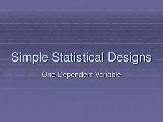
Simple Statistical Designs. One Dependent Variable. If I have one Dependent Variable, which statistical test do I use?. Is your Dependent Variable (DV) continuous?. YES. NO. Is your Independent Variable (IV) continuous?. Is your Independent Variable (IV) continuous?. YES. NO. YES. NO.

E N D
Simple Statistical Designs One Dependent Variable
If I have one Dependent Variable, which statistical test do I use? Is your Dependent Variable (DV) continuous? YES NO Is your Independent Variable (IV) continuous? Is your Independent Variable (IV) continuous? YES NO YES NO Correlation or Linear Regression Logistic Regression Chi Square Do you have only 2 treatments? YES NO T-test ANOVA
Chi Square (χ2) • Non-parametric: no parameters estimated from the sample • Chi Square is a distribution with one parameter: degrees of freedom (df). • Positively skewed but skew decreases with df. • Mean is df • Goodness-of-fit and Independence Tests
Chi-Square Goodness of Fit Test • How well do observed proportions or frequencies fit theoretically expected proportions or frequencies? • Example: Was test performance better than chance? χ2 =Σ(Observed – Expected)2 df = # groups -1 Expected
Chi Square Test for Independence • Is distribution of one variable contingent on another variable? • Contingency Table • df = (#Rows -1)(#Columns-1) • Example: Ho: depression & gender are independent H1: depression and gender are not independent
Chi Square Test for Independence Same χ2formula except expected frequencies are derived from the row and column totals: cell proportion X Total = (30/100)(50/100)(100) χ2 = (10-15)2+ (20-15)2+ (40-35)2+ (30-15)2= 4.76 15 15 35 35 Critical χ2 with 1 df = 3.84 at p=.05 Reject Ho : depression and gender are NOT independent
Assumptions of Chi Square • Independence of observations • Categories are mutually exclusive • Sampling distribution in each cell is normal • Violated if expected frequencies are very low (<5); robust if > 20. • Fisher’s Exact Test can correct for violations of these assumptions in 2x2 designs.
Recall the Bivariate Distribution r = -.17 p=.09
Interpretation of r • Slope of best fitting straight regression line when variables are standardized • measure of the strength of the relationship between 2 variables • r2 measures proportion of variability in one measure that can be explained by the other • 1-r2 measures the proportion of unexplained variability.
Simple Regression • Prediction: What is the best prediction of variable X? • Regress Y on X (i.e. regress outcome on predictor) • CorrelationRegression.html
The fit of a straight line • The straight line is a summary of a bivariate distribution • Y = a + bx + ε • DV = intercept + slope(IV) + error • Least Squares Fit: minimize error by minimizing sum of squared deviations: Σ(Actual Y - Predicted Y)2 • Regression lines ALWAYS pass through the mean of X and mean of Y
b • Slope: the magnitude of change in Y for a 1 unit change in X • Beta= b = r(SDy/SDx) • Because of this relationship: Zy = r Zx • Standardized beta: if X and Y are converted to Z scores, this would be the beta – not interpretable as slope.
Residuals • The error in the estimate of the regression line • Mean is always 0 • Residual plots are very informative – tell you how well your line fits the data • Linear Regression Applet
Assumptions & ViolationsLinear Regression Applet • Homoscedasticity: uniform variance across whole bivariate distribution. • Bivariate outlier: not outlier on either X or Y • Influential Outliers: ones that move the regression line • Y is Independent and Normally distributed at all points along line (residuals are normally distributed) • Omission of important variables • Non-linear relationship of X and Y • Mismatched distributions (i.e. neg skew and pos skew – but you already corrected those with transformations, right?) • Group membership (i.e. neg r within groups, pos r across groups)
Logistic Regression • Continuous predictor(s) but DV is now dichotomous. • Predicts probability of dichotomous outcome (i.e. pass/fail, recover/relapse) • Not least squares but maximum likelihood estimate • Fewer assumptions than multiple regression • “Reverse” of ANOVA • Similar to Discriminant Function Analysis that predicts nominal-scaled DVs of > 2 categories
T-test • Similar to Z but with estimates instead of actual population parameters mean1 – mean2 pooled within-group SD • One- or two-tailed, use one-tailed if you can justify through hypothesis - more power • Effect size is Cohen’s d
One Sample t-test Compare mean of one variable to a specific value (i.e. Is IQ in your sample different from national norm?) Sample mean – 100 15
Independent Sample t-test • Are 2 groups significantly different from each other? • Assumes independence of groups, normality in both populations, and equal variances (although T is robust against violations of normality). • Pooled variance = mean of variances (or weighted by df if variances are unequal) • If N’s unequal, use Welch t-test
Dependent Samples t-test(aka Paired Samples t-test) • Dependent Samples: • Same subjects, same variables • Same subjects, different variables • Related subjects, same variables (i.e. mom and child) • More powerful: pooled variance (denominator) is smaller • But fewer df, higher critical t
Univariate (aka One-Way) ANOVA Analysis of Variance • 2 or more levels of a factor • ANOVA tests Ho that means of each level are equal • Significant F only indicates that the means are not equal.
F • F statistic = t2 = Between Group Variance = signal Within Group Variance noise Robust against violations of normality unless n is small Robust against violations of homogeneity of variances unless n’s are unequal If n’s are unequal, use Welch F’ or Brown-Forsythe F*
Effect size • Large F does NOT equal large effect • Eta Squared (η2): Sum-of-Squares between Sum-of-squares Total Variance proportion estimate Positively biased – OVERestimates true effect • Omega squared (ω2) adjusts for within factor variability and is better estimate
Family-wise error • F is a non-directional, omnibus test and provides no info about specific comparisons between factors. In fact, a non-significant omnibus F does not mean that there are not significant differences between specific means. • However, you can’t just run a separate test for each comparison – each independent test has an error rate (α). • Family-wise error rate = 1 – (1- α)c, where c = # comparisons • Example: 3 comparisons with α=.05 1 – (1- .05)3 = .143
Contrasts • A linear combination of contrast coefficients (weights) on the means of each level of the factor To contrast the Control group against the Drug 1 group, the contrast would look like this: Contrast = 1(Control) + (-1)(Drug 1) + 0(Drug 2)
Unplanned (Post-hoc) Contrasts • Risk of Family-wise error • Correct with: • Bonferoni inequailty: multiply α by # comparisons • Tukey’s Honest Significant Difference (HSD): minimum difference between means necessary for significance • Scheffe test: critical F’ = (#groups-1)(F) ultraconservative
Planned Contrasts • Polynomial: linear, quadratic, cubic, etc. pattern of means across levels of the factor • Orthogonal: sum of contrast coefficients (weights) equals 0. • Non-orthogonal: sum of contrast coefficients does not equal 0
Polynomial Contrasts(aka Trend Analysis) • Special case of orthogonal contrasts but IV must be ordered (e.g. time, age, drug, dosage) Linear Quadratic Cubic Quartic
Orthogonal Contrasts • Deviation : Compares the mean of each level (except one) to the mean of all of the levels (grand mean). Levels of the factor can be in any order.
Orthogonal Contrasts Simple: Compares the mean of each level to the mean of a specified level. This type of contrast is useful when there is a control group. You can choose the first or last category as the reference.
Orthogonal Contrasts Helmert : Compares the mean of each level of the factor (except the last) to the mean of subsequent levels combined.
Orthogonal Contrasts Difference : Compares the mean of each level (except the first) to the mean of previous levels. (aka reverse Helmert contrasts.)
Orthogonal Contrasts Repeated : Compares the mean of each level (except the last) to the mean of the subsequent level.
Non-orthogonal Contrasts • Not used often • Dunn’s test (Bonforoni t): controls for family-wise error rate by multiplying αby the number of comparisons. • Dunnett’s test: use t-test but critical t values come from a different table (Dunnett’s) that restricts family-wise error.