Locally Linear Support Vector Machines

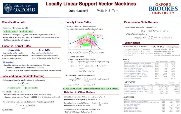
1. Locally Linear Support Vector Machines Ľubor Ladický Philip H.S. Torr Classification task Locally Linear SVMs Extension to Finite Kernels • The decision boundary should be smooth • Approximately linear in a sufficiently small region • The finite kernel classifier takes the form : • Weights W and b obtained as : Given : { [x1, y1], [x2, y2], … [xn, yn] } xi - feature vector yi {-1, 1} - label • The task is : To design y = H(x) that predicts a label y for a new vector x • Many approaches proposed (Boosting, Random Forests, Neural Nets, SVMs, ..) • SVM seems to dominate the others Experiments • CALTECH-101 (15 samples per class) • Coordinates evaluated on kNN (k = 5) • Approximated Intersection kernel used • Spatial pyramid of BOW features • Coordinates evaluated based on image histograms Linear vs. Kernel SVMs • MNIST, LETTER & USPS datasets • Anchor points obtained using K-means clustering • Coordinates evaluated on kNN (k = 8) (slow part) • Coordinates obtained using weighted inverse distance • Raw data used • Kernel SVMs • Slow training and evaluation • Not feasible for large scale data sets • Better performance for hard problems • Linear SVMs • Fast training and evaluation • Applicable to large scale data sets • Low discriminative power • Curvature is bounded • Functions wi(x) and b(x) are Lipschitz • wi(x) and b(x)can be approximated using local coding • MNIST • Motivation : • Exploiting manifold learning techniques to design an SVM with • Good trade-off between the performance and speed • Scalability to large scale data sets (solvable with stochastic gradient descent) • Weights W and biases b are obtained as : • where Local coding for manifold learning • Points approximated as a weighted sum of anchor points • Coordinates obtained using : • Distance based methods (Gemert et al. 2008, Zhou et al. 2009) • Reconstruction methods (Roweis et al.2000, Yu et al. 2009, Gao et al. 2010) • USPS / LETTER v – anchor points v(x) - coordinates γ [xk, yk] – training samples λ- regularisation weight S – number of samples Relation to Other Models • Generalisation of Linear SVM on x : • representable by W = (ww ..)T and b = (b’ b’ ..)T • Generalisation of linear SVM on γ: • representable by W = 0 andb = w • Generalisation of model selecting Latent(MI) SVM : • Representable by γ= (0, 0, .., 1, .. 0) • CALTECH-101 • For a normalised coding any Lipschitz function f can be approximated : • (Yu et al. 2009)