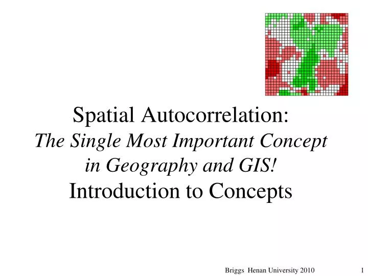
Spatial Autocorrelation: The Single Most Important Concept in Geography and GIS! Introduction to Concepts

1. Spatial Autocorrelation:The Single Most Important Concept in Geography and GIS!Introduction to Concepts Briggs Henan University 2010

2.  Spatial Statistics  Descriptive Spatial Statistics: Centrographic Statistics (This time) single, summary measures of a spatial distribution - Spatial equivalents of mean, standard deviation, etc.. Inferential Spatial Statistics: Point Pattern Analysis (Next time) Analysis of point location only--no quantity or magnitude (no attribute variable) --Quadrat Analysis --Nearest Neighbor Analysis, Ripley’s K function Spatial Autocorrelation (Weeks 5 and 6) One attribute variable with different magnitudes at each location The Weights Matrix Global Measures of Spatial Autocorrelation (Moran’s I, Geary’s C, Getis/Ord Global G) Local Measures of Spatial Autocorrelation (LISA and others) Prediction with Correlation and Regression (Week 7) Two or more attribute variables Standard statistical models Spatial statistical models Briggs Henan University 2010

3. Point Pattern Analysis (PPA) and Spatial Autocorrelation (SA) : differences and similarities Point Pattern Analysis (last time) --points only, and only their location --there is no “magnitude” value Spatial Autocorrelation: (this time) --points and polygons, with different “magnitudes” -- there is an attribute variable. --income, rainfall, crime rate, etc. Briggs Henan University 2010

4. Spatial AutocorrelationMany ways to define it! 1. The confirmation of Tobler’s first law of geography Everything is related to everything else, but near things are more related than distant things. 2. Using similarity The degree to which characteristics at one location are similar (or dissimilar) to those nearby. 3. Using probability Measure of the extent to which the occurrence of an event in one geographic area makes more probable, or less probable, the occurrence of a similar event in a neighboring geographic area. 4. Using correlation Correlation of a variable with itself through space. The correlation between an observation’s value on a variable and the value of near-by observations on the same variable Lets look at these in more detail.

5. Spatial Autocorrelation:1. Tobler’s Law The confirmation of Tobler’s first law of geography*: Everything is related to everything else, but near things are more related than distant things. The single most important concept in geography and GIS! *Tobler W., (1970) "A computer movie simulating urban growth in the Detroit region". Economic Geography, 46(2): 234-240 Briggs Henan University 2010

6. Positive Spatial Autocorrelation Spatial Autocorrelation Spatial: On a map Auto: Self Correlation: Degree of relative similarity Positive: similar values cluster together on a map Negative Spatial Autocorrelation Source: Dr Dan Griffith, with modification Negative: dissimilar (different) values cluster together on a map Briggs Henan University 2010

7. 2002 population density Positive spatial autocorrelation - high values surrounded by nearby high values - intermediate values surrounded by nearby intermediate values - low values surrounded by nearby low values

8. competition for space Negative spatial autocorrelation - high values surrounded by nearby low values - intermediate values surrounded by nearby intermediate values - low values surrounded by nearby high values Grocery store density

9. Spatial Autocorrelation:more ways to describe it 2. Based on Similarity The degree to which characteristics at one location are similar to (or different from) those nearby. Similar to = positive spatial autocorrelation Different from (dissimilar) = negative spatial autocorrelation Positive spatial autocorrelation much more common than negative Briggs Henan University 2010

10. Spatial Autocorrelation Exists Everywhere! POLLUTION MONITORING SATELLITE IMAGE HOUSEHOLD SAMPLING AGRICULTURAL EXPERIMENT Briggs Henan University 2010

11. UNIFORM/ DISPERSED CLUSTERED Spatial Autocorrelation:more ways to describe it • Based on Probability Measure of the extent to which the occurrence of an event in one geographic unit (polygon) makes more probable, or less probable, the occurrence of a similar event in a neighboring unit. Do you recognize this from earlier discussion? It’s the same concept as clustered, random, dispersed! high negative spatial autocorrelation no spatial autocorrelation* high positive spatial autocorrelation Dispersed Pattern Random Pattern Clustered Pattern Briggs Henan University 2010

12. Even More Ways to Describe SA 4. Using correlation Correlation of a variable with itself through space. The correlation between an observation’s value on a variable and the value of near-by observations on the same variable. Correlation = “similarity”, “association”, or “relationship” Scatter diagram Crime rate in near-by area Crime rate in an area Briggs Henan University 2010

13. Scatter Diagram: how is it different? Spatial Autocorrelation: shows the association or relationship between the same variable in “near-by” areas. Standard Statistics: shows the association or relationship between two different variables Each point is a geographic location Education “next door” income In a neighboring or near-b y area education education Briggs Henan University 2010

14. Why is Spatial Autocorrelation Important? Two reasons • Spatial autocorrelation is important because it implies the existence of a spatial process • Why are near-by areas similar to each other? • Why do high income people live “next door” to each other? • These are GEOGRAPHICAL questions. • They are about location 2. It invalidates most traditional statistical inference tests • If SA exists, then the results of standard statistical inference tests may be incorrect (wrong!) • We need to use spatial statistical inference tests Infer Population Sample Create Pattern Processes Briggs Henan University 2010

15. Why are standard statistical tests wrong? • Statistical tests are based on the assumption that the values of observations in each sample are independent of one another • spatial autocorrelation violates this • samples taken from nearby areas are related to each other and are not independent Implies a relationship between nearby observations Values near each other are similar in magnitude. Briggs Henan University 2010

16. Why are standard statistical tests wrong?Example for the correlation coefficient (r) What is the correlation coefficient (r)? • The most common statistic in all of science • measures the strength of the relationship (or “association”) between two variables e.g. income and education • Varies on a scale from –1 thru 0 to +1 +1 implies a perfect positive association • As values go up () on one, they also go up () on the other • income and education 0 implies no association -1 implies perfect negative association • As values go up on one () , they go down () on the other • price and quantity purchased • Full name is the Pearson Product Moment correlation coefficient, () () () () -1 0 +1 Briggs Henan University 2010

17. Examples of Scatter Diagrams and the Correlation Coefficient Positive r = 1 r = 0.72 Income perfect positive strong positive Education r = 0.26 Negative weak positive r = -0.71 r = -1 Quantity perfect negative strong negative Price Briggs Henan University 2010

18. Why are standard statistical tests wrong?Example for the correlation coefficient (r) If Spatial Autocorrelation exists: • Correlation coefficients appear to be bigger than they really are, and • They are more likely to be found “statistically significant” You are “fooled twice”: --you are more likely to incorrectly conclude a relationship exists when it does not --You believe that the relationship is stronger than it really is Briggs Henan University 2010

19. Why are standard statistical tests wrong?Example for the correlation coefficient (r) If Spatial Autocorrelation exists: • Correlation coefficients bigger than they really are • because income and education are similar in near by areas • Correlation coefficient is “biased upward” • Also, more likely to appear “statistically significant” • standard error is smaller because spatial autocorrelation “artificially” reduces variability • there is actually more variability than it appears • “exagerated precision” Briggs Henan University 2010

20. Measuring Spatial Autocorrelation: the problem of measuring “nearness” or “proximity” Briggs Henan University 2010

21. Measuring Spatial Autocorrelation:the problem of measuring “nearness” To measure spatial autocorrelation, we must know the “nearness” of our observations • Which points or polygons are “ near” or “next to” other points or polygons? • Which provinces are near Henan? • How measure this? Seems simple and obvious, but it is not! Briggs Henan University 2010

22. Measuring Spatial Autocorrelation:the Spatial Weights matrix • Wij the spatial weights matrix measures the relative location of all points i and j, • Different methods of calculating Wij can result in different values for autocorrelation and different conclusions from statistical significance tests! Wij ? Briggs Henan University 2010

23. Measuring Relative Spatial Location:Contiguity and Distance Two methods for measuring nearness 1. Weights based on Contiguity--binary (0,1) • If zone j is next to zone i, it receives a weight of 1 • otherwise it receives a weight of 0, • It is essentially excluded • But what constitutes contiguity? Not as easy as it seems! 2. Weights based on Distance—continuous variable • Measure the actual distance between points, or between polygon centroids • But what measure do we use, and • distance to what points -- All? Some? Briggs Henan University 2010

24. Spatial neighbors based on contiguity* (adjacency) * Shares common border rook queen Hexagons Irregular Which use? • Sharing a border or boundary • Rook: sharing a border • Queen: sharing a border or a point Briggs Henan University 2010

25. Spatial weights matrix for Rook case associated geographic connectivity/ weights matrix 4 areal units 4x4 matrix W = Common border • Matrix contains a: • 1 if share a border • 0 if do not share a border Briggs Henan University 2010

26. X Problem Situations for Irregular PolygonsMany! “Close” but no common border • Include polygons which have a centroid within the “convex hull” for the centroids of polygons that do share a common border Length of border • Is Shanxi “as close to” Nei Mongol as to Henan? • Base “closeness” on proportion of shared border, not just one (1) or zero (0) • wij = border lengthij /border lengthj) Briggs Henan University 2010

27. Measuring Contiguity: Lagged ContiguityShould we include second order contiguity? 1st order Nearest neighbor rook hexagon queen 2nd order Next nearest neighbor Briggs Henan University 2010

28. Formats for Weights Matrix Raw versus row standardized Full contiguity versus sparse contiguity Briggs Henan University 2010

29. Row-standardized geographic contiguity matrices Divide each number by the row sum Total number of neighbors --some have more than others Row standardized --usually use this Briggs Henan University 2010

30. Queens Case Full Contiguity Matrix for US States • Column headings not shown (same as rows) • Principal diagonal has 0s (blanks) • other 0s omitted for simplicity • Can be very large, thus inefficient to use. Briggs Henan University 2010

31. Queens Case Sparse Contiguity Matrix for US States • Ncount is the number of neighbors for each state • Max is 8 (Missouri and Tennessee) • Sum of Ncount is 218 • Number of common borders (joins) • ncount / 2 = 109 • N1, N2… FIPS codes for neighbors Briggs Henan University 2010

32. Challenge for You • Which China province has the most neighbors? • How many does it have? • Create contiguity matrices for the Provinces of China • Can be done with GeoDA or with ArcGIS • Or you can do it “by hand” • Use the software to see if you get it correct Briggs Henan University 2010

33. Weights Based on Distanceagain, not that simple • Functional Form to use? • Distance metric to use ? • Which points/polygons to include? • How measure distance between polygons? Briggs Henan University 2010

34. Weights Based on Distance 1. Functional Form • We want “nearness” not distance • Most common choice is the inverse (reciprocal) of the distance between locations i and j (wij = 1/dij) • Other functions also used • inverse of squared distance (wij =1/dij2), or • negative exponential (wij = e-d or wij = e-d2) distance nearness Briggs Henan University 2010

35. Weights Based on Distance • 2. Distance metric • 2-D Cartesian distance via Pythagorus • Use for projected data • 3-D Spherical distance via spherical coordinates • Cos d = (sin a sin b) + (cos a cos b cos P) • where: d = arc distance • a = Latitude of A • b = Latitude of B • P = degrees of long. A to B • Use for unprojected data • possible distance metrics: • Euclidean straight line/airline • city block/manhattan metric • distance through network Appropriate if within a city Briggs Henan University 2010

36. Weights based on Distance 3. What points/polygons to include? • Distances to all points/polygons? • If use all, may make it impossible to solve necessary equations: matrix too big • May not make theoretical sense: effects may only be ‘local’ • Is Henan influenced by Xinjiang? • Include distance to only the “nth” nearest neighbors • How many is n? First? Second? • Include distances to locations only within a buffer distance

37. Weights based on Distance 4. Measuring distance between polygons • distances usually measured centroid to centroid, but • could be measured from boundary of one polygon to centroid of others • could be measured between the two closest boundary points • adjustment required for contiguous polygons since distance for these would be zero Briggs Henan University 2010

38. Many decisions!Many challenges! That is what makes research fun! Briggs Henan University 2010

39. What have we learned today? • The concept of spatial autocorrelation. • “Near things are more similar than distant things” • The use of the weights matrix Wijto measure “nearness” • The difficulty of measuring “nearness” • That is a surprise! Next Time • Measures of Spatial Autocorrelation • Join Count statistic --Geary’s C • Moran’s I --Getis-Ord G statistic Briggs Henan University 2010

40. Challenge for You • Which China province has the most neighbors? • How many does it have? • Create contiguity matrices for the Provinces of China • Can be done with GeoDA or with ArcGIS • Or you can do it “by hand” • Use the software to see if you get it correct Briggs Henan University 2010

41. Appendix: A Note on Sampling Assumptions • Another factor which influences results from these tests is the assumption made regarding the type of sampling involved: • Free (or normality) sampling • Analogous to sampling with replacement • After a polygon is selected for a sample, it is returned to the population set • The same polygon can occur more than one time in a sample • Non-free (or randomization) sampling • Analogous to sampling without replacement • After a polygon is selected for a sample, it is not returned to the population set • The same polygon can occur only one time in a sample • The formulae used to calculate test statistics (particularly the standard error) differ depending on which assumption is made • Generally, the formulae are substantially more complex for randomization sampling—unfortunately, it is also the more common situation! • Usually, assuming normality sampling requires knowledge about larger trends from outside the region or access to additional information within the region in order to estimate parameters. Briggs Henan University 2010

42. Briggs Henan University 2010