Download
1 / 26
300 likes | 355 Views
Wind Driven Circulation I: Ekman Layer. Scaling of the horizontal components. . (accuracy, 1% ~ 1‰). Rossby Number. Vertical Ekman Number. R o and E v are non-dimensional parameters. Geostrophic balance => R o , E v <<1. (1). (2). The parameterized turbulent momentum transports are.

E N D
Scaling of the horizontal components (accuracy, 1% ~ 1‰) Rossby Number Vertical Ekman Number Ro and Ev are non-dimensional parameters. Geostrophic balance => Ro, Ev <<1
(1) (2) The parameterized turbulent momentum transports are We can also write the momentum equations in more form etc At the sea surface (z=0), the turbulent transport is wind stress.
Surface wind stress • Approaching sea surface, the geostrophic balance is broken, even for large scales. • The major reason is the influences of the winds blowing over the sea surface, which causes the transfer of momentum (and energy) into the ocean through turbulent processes. • The surface momentum flux into ocean is called the surface wind stress ( ), which is the tangential force (in the direction of the wind) exerting on the ocean per unit area (Unit: Newton per square meter) • The wind stress effect can be constructed as a boundary condition to the equation of motion as
In neutral condition, von Karman logarithmic law of wall The surface momentum flux is zo is aerodynamic roughness length If we choose wind measurement at a certain height, e.g., 10m above the sea surface, the bulk formula is is 10m neutral drag coefficient
Wind stress Calculation • Direct measurement of wind stress is difficult. • Wind stress is mostly derived from meteorological observations near the sea surface using the bulk formula with empirical parameters. • The bulk formula for wind stress has the form Where is air density (about 1.2 kg/m3 at mid-latitudes), V (m/s), the wind speed at 10 meters above the sea surface, Cd, the empirical determined drag coefficient
Drag Coefficient Cd • Cd is dimensionless, ranging from 0.001 to 0.0025 (A median value is about 0.0013). Its magnitude mainly depends on local wind stress and local stability. • Cd Dependence on stability (air-sea temperature difference). More important for light wind situation For mid-latitude, the stability effect is usually small but in tropical and subtropical regions, it should be included. • CdDependence on wind speed.
Cd dependence on wind speed in neutral condition Large uncertainty between estimates (especially in low wind speed). Lack data in high wind
Observations of the drag coefficient as a function of wind speed U10 ten meters above the sea. The solid line is from the formula proposed by Yelland and Taylor (1996). The dotted line is 1000CD=0.44 + 0.063U10 proposed by Smith (1980) and the dashed line follows from Charnock(1995). Triangles are values measured by Powell, Vickery, and Reinhold (2003). From Stetart (2008). The more recently published formula by Yelland and Taylor (1996) for neutrally stable boundary layer: (3 ≤ U10 ≤ 6 m/s) (6 ≤ U10 ≤ 26 m/s)
Annual Mean surface wind stress Unit: N/m2, from Surface Marine Data (NODC)
December-January-February mean wind stress Unit: N/m2, from Surface Marine Data (NODC)
December-January-February mean wind stress Unit: N/m2, from Scatterometer data from ERS1 and 2
June-July-August mean wind stress Unit: N/m2, from Surface Marine Data (NODC)
June-July-August mean wind stress Unit: N/m2, Scatterometers from ERS1 and 2
Assumption for the Ekman layer near the surface • Az=const • Steady state (steady wind forcing for long time) • Small Rossby number • Large vertical Ekman Number • Homogeneous water (=const) • f-plane (f=const) • no lateral boundaries (1-d problem) • infinitely deep water below the sea surface
Ekman layer • Near the surface, there is a three-way force balance Coriolis force+vertical dissipation+pressure gradient force=0 Geostrophic current let Ageostrophic (Ekman) current (note that VE is not small in comparison to Vg in this region) then
The Ekman problem (1) (2) Boundary conditions At z=0, As z- ,. , . (3) (5) (6) (4) Let (complex variable), take (1) + i(2), we have Since (7)
Take (3) + i (4), we have (3) z=0, (4) Define (8) (5) Take (5) + i (6), we have As z-, (9) (6) Group equations (7), (8), and (9) together, we have (7) At z=0, (8) (9) As z-
Assume the solution for (7) has the following form Take into We have If f > 0, If f < 0, In above derivations, we have used the following equality: For f > 0, the general solution of (7) can be written as
(8) As z- Therefore, B=0 because grow exponentially as z- and Then At z=0, (9) then and The final solution to (7), (8), (9) is
Given Set , where and Also note that We have Current Speed: (=0, eastward) Phase (direction):