Download
1 / 74
760 likes | 808 Views
Network Topology. ELEG 667-013 Spring 2003. Outline:. Why Network Topology is Important ? Modeling Internet Topology Complex Networks Scale-free Networks Power-laws of the Web Search in power-law networks: GNUTELLA, a P2P example. Why Topology is Important ?.

E N D
Network Topology ELEG 667-013 Spring 2003
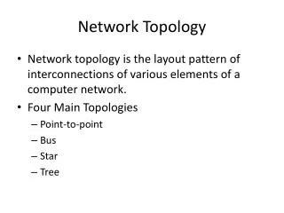
Outline: • Why Network Topology is Important ? • Modeling Internet Topology • Complex Networks • Scale-free Networks • Power-laws of the Web • Search in power-law networks: GNUTELLA, a P2P example.
Why Topology is Important ? • Design Efficient Protocols • Solve Internetworking Problems: • - routing • - resource reservation • - administration • Create Accurate Model for Simulation • Derive Estimates for Topological Parameters • Study Fault Tolerance and Anti-Attack Properties
Modeling Internet Topology [1]: • Graph representation • Router-level modeling - vertices are routers • edges are one-hop IP connectivity • Domain- (AS-) level model (high degree of abstraction) - vertices are domains (ASes) • - edges are peering relationships • Nodes can be assigned numbers rep. e.g. buffer capacity • Edges migth have weights rep. e.g. – prop. delay, bandwidth capacity.
Modeling Internet Topology [1]: transit domains domains/autonomous systems exchange point border routers peering hosts/endsystems routers stub domains lowly worm access networks
Barabasi Albert Model (BA Model): • Basis for most current topology generators • Very simplistic model • Network evolves in size over time. • Preferential Connectivity • Probability that a newly added node will attach to node ‘i’ • Many extensions.
Waxman Model: • Router level model • Nodes placed at random in 2D space with dimension L • Probability of edge (u,v): • a*e(-d / (bL) ), where d is Euclidean distance (u,v), a and b are constants • Models locality • no sense of backbone or hierarchy • does not guarantee connected network • as #nodes ↑ the #links ↑ proportionally u d(u,v) v
Transit-Stub Model: • Router level model • Transit domains • placed in 2D space • populated with routers • connected to each other • Stub domains • placed in 2D space • populated with routers • connected to transit domains • Models hierarchy • Edge count, guaranteed connectivity
Transit-Stub Model: • No concept of a ‘host’ – all nodes are routers. • Two level hierarchy • First generate a number of transit domains, then generate a set of stub networks. • Given average edge-count, produce a random graph, making sure that it is connected.
Inet: • Generate degree sequence • Build spanning tree over nodes with degree larger than 1, using preferential connectivity • randomly select node u not in tree • join u to existing node v with probability d(v)/d(w) • Connect degree 1 nodes using preferential connectivity • Add remaining edges using preferential connectivity
BRITE: • Generate small backbone, with nodes placed: • randomly or • concentrated (skewed) • Add nodes one at a time (incremental growth) • New node has constant # of edges connected using: • preferential connectivity and/or • locality
Complex Networks: • Two limiting-case topologies have been extensively considered in the literature [4],[5].: • regular network (lattice), the chosen topology of innumerable physical models such as the Ising model or percolation. • random graph,studied in mathematics and used both in natural and social sciences. Properties studied in detail by Pal Erdos. • Most of Erdos’ work concentrated on the case in which the number of vertices is kept constant but the total number of links between vertices increases: the Erdös-Rényi result states that for many important quantities there is a percolation-like transition at a specific value of the average number of links per vertex.
Complex Networks: • random networks are used in: • Physics: in studies of dynamical problems, spin models and thermodynamics, random walks, and quantum chaos. • Economics and social sciences: to model interacting agents.
Complex Networks: • In contrast to these two limiting topologies, empirical evidence suggests that many biological, technological or social networks appear to be somewhere in between these extremes. • many real networks seem to share with regular networks the concept of neighborhood, which means that if vertices i and j are neighbors then they will have many common neighbors --- which is obviously not true for a random network. • On the other hand, studies on epidemics show that it can take only a few ``steps'' on the network to reach a given vertex from any other vertex. This is the foremost property of random networks, which is not fulfilled by regular networks.
Complex Networks: • The Watts-Strogatz model [5]. : • To bridge the two limiting cases, Watts and Strogatz [Nature 393, 440 (1998)] have introduced a new type of network which is obtained by randomizing a fraction p of the links of the regular network. • Initial structure (p=0) is the one-dimensional regular network where each vertex is connected to its z nearest neighbors. • For 0 < p < 1, we denote these networks disordered. • for the case p=1, we have a completely random network.
Complex Networks: • Watts and Strogatz report that for a small value of the parameter p, there is an onset of “small-world” behavior. • It is characterized by the fact that the distance between any two vertices is of the order of that for a random network and, at the same time, the concept of neighborhood is preserved. • The effect of a change in p is extremely nonlinear, where a very small change in the connectivity of the network leads to a dramatic change in the distance between different pairs of vertices.
Complex Networks: • The scientific question we are trying to answer is: Does the onset of the small-world behavior occurs at a given value of p or does it occur for a value of the system size n which depends on p? • To investigate this question, we need to look at the behavior of the system as a function of p for different values of n.
Complex Networks: • The appearance of the small-world behavior is not a phase-transition but a crossover phenomena. • The average distance l is: l (n,p) ~ n* F ( n / n* ) where: F(u << 1) ~ u, and F(u >> 1) ~ln u, and n* is a function of p. • When the average number of rewired links, pnz/2, is much less than one, the network should be in the large-world regime. On the other hand, when pnz/2 >> 1, the network should be a small-world.
Scale-free networks: • It was proposed by Barabási and Albert that real-world networks in general are scale-free networks. • Scale-free networks have a distribution of connectivities that decays with a power-law tail. • Scale-free networks emerge in the context of a growing network in which new vertices connect preferentially to the more highly connected vertices in the network. Scale free networks are also small-world networks because (i) they have clustering coefficients much larger than random networks, and (ii) their diameter increases logarithmically with the number of vertices n.
What are Power Laws ? • Distribution that fits : • Characteristic property of “Scale free networks” • Occur very often in Complex Systems literature. • Many complicated real world networks obey power laws
Implications of Power Laws: • Majority of nodes have small connectivity. • Few nodes have very large connectivity. • Good resistance to random failure. • Small resistance to planned attack. • Could imply existence of some hierarchy (all real world power law networks support this). • However, it is not clear whether Power Law Hierarchy
Origin of Power Law: • Power laws are an observed (empirical) phenomenon. • The mechanisms that produce these can only be guessed at (for now!) • Very typical in self organizing systems and chaotic systems.
Scale-free networks: • Scale-free networks: • (a) the neuronal network of the worm C. elegans. • (b) world-wide web. • (c) the network of citations of scientific papers.
Scale-free networks: • broad-scale networks: or truncated scale-free networks, characterized by a connectivity distribution that has a power-law regime followed by a sharp cut-off, like an exponential or Gaussian decay of the tail. • single-scale networks: characterized by a connectivity distribution with a fast decaying tail, such as exponential or Gaussian • Aging of the vertices: The vertex is still part of the network and contributing to network statistics, but it no longer receives links. The aging of the vertices thus limits the preferential attachment preventing a scale-free distribution of connectivities. • Cost of adding links to the vertices or the limited capacity of a vertex: physical costs of adding links and limited capacity of a vertex will limit the number of possible links attaching to a given vertex.
Power-laws of the Web [2].: • How many links on a page (outdegree)? • How many links to a page (indegree)? • Probability that a random page has k other pages • pointing to it is ~k-2.1 (Power law) • Probability that a random page points to k other pages is • ~k-2.7 (Power law)
Search in power-law networks: GNUTELLA [3]. • Most of the P2P networks display a power-law distribution in their node degree. This distribution reflects the existence of a few nodes with very high degree and many with low degree. • In P2P networks, the name of the target file may be known, but due to the network’s ad hoc nature, the node holding the file may not be known until a real-time search is performed. • A simple strategy to locate files, implemented by NAPSTER, is to use a central server that contains an index of all the files every node is sharing as they join the network. • GNUTELLA and FREENET do not use a central server.
Search in power-law networks: GNUTELLA [3]. • GNUTELLA is a peer-to-peer file-sharing system that treats • all client nodes as functionally equivalent and lacks a central • server that can store file location information. This is advantageous • because it presents no central point of failure. • The obvious disadvantage is that the location of files is unknown. • When a user wants to download a file, he sends a query to • all the nodes within a neighborhood of size ttl, the time to • live assigned to the query. Every node passes on the query to • all of its neighbors and decrements the ttl by one. In this • way, all nodes within a given radius of the requesting node • will be queried for the file, and those who have matching • files will send back positive answers.
Search in power-law networks: GNUTELLA [3]. • This broadcast method will find the target file quickly, • given that it is located within a radius of ttl. However, broadcasting • is extremely costly in terms of bandwidth. • Such a search strategy does not scale well. As query traffic increases linearly with the size of GNUTELLA graph, nodes • become overloaded.
Search in power-law networks: GNUTELLA [3]. • Typically, a GNUTELLA client wishing to join the network • must find the IP address of an initial node to connect to. • Currently, ad hoclists of ‘‘good’’ GNUTELLA clients exist. • It is reasonable to suppose that this ad hocmethod of • growth would bias new nodes to connect preferentially to • nodes that are already fairly well connected, since these • nodes are more likely to be ‘‘well known.’’ • Based on models of graph growthwhere the ‘‘rich get richer,’’ the power-law connectivity of ad hocpeer-to-peer networks may • be a fairly general topological feature.
Search in power-law networks: GNUTELLA [3]. • By passing the query to every single node in the network, • the GNUTELLA algorithm fails to take advantage of the connectivity distribution [3]. • To take advantage of the power-law distribution, we can modify • each node to keep lists of files stored in first and second neighbor. • Instead of passing the query to every node, now we can pass it only to the nodes with highest connectivity. • High degree nodes are presumably high bandwidth node that can handle the query traffic.
Outline: Internet Structure &Organization • Internet Hierarchical Structure • ISPs, interconnection and organization [ref. 7]. • POP Architecture and Load Balancing • ISP Architecture [ref. 7]. in detail • Topology Mapping Tool: Rocketfuel[ref. 8] • Discussion ELEG 667-013 Spring 2003
Basic Architecture: NAPs and national ISPs • The Internet has a hierarchical structure. • At the highest level are large national Internet Service Providers that interconnect through Network Access Points (NAPs). • There are about a dozen NAPs in the U.S., run by common carriers such as Sprint and Ameritech, and many more around the world. • Regional ISPs interconnect with national ISPs which provide services to local ISPs who, in turn, sell access to individuals.
Basic Architecture: MAEs and local ISPs • As the number of ISPs has grown, a new type of network access point, called a metropolitan area exchange (MAE) has arisen. • There are about 50 such MAE around the U.S. today. • Sometimes large regional and local ISPs also have access directly to NAPs.
Internet Packet Exchange Charges • ISP at the same level usually do not charge each other for exchanging messages. • This is called peering. • Higher level ISPs, however, charge lower level ones (national ISPs charge regional ISPs which in turn charge local ISPs) for carrying Internet traffic. • Local ISPs, of course, charge individuals and corporate users for access.
Connecting to an ISP • ISPs provide access to the Internet through a Point of Presence (POP). • Individual users access the POP through a dial-up line using the PPP protocol. • The call connects the user to the ISP’s modem pool, after which a remote access server (RAS) checks the userid and password. • Once logged in, the user can send TCP/IP/[PPP] packets over the telephone line which are then sent out over the Internet through the ISP’s POP.
Connecting to an ISP (contd.) Corporate users might access the POP using a T-1, T-3 or ATM OC-3 connections provided by a common carrier. T-1 and T-3 lines connect to the ISP POP’s CSU/DSU device. Channel Service Unit/Data Service Unit. The CSU is a device that connects a terminal to a digital line. The DSU is a device that performs protective and diagnostic functions for a telecommunications line. . Typically, the two devices are packaged as a single unit. You can think of it as a very high-powered and expensive modem. Such a device is required for both ends of a T-1 or T-3 connection, and the units at both ends must be set to the same communications standard.
Inside an ISP Point of Presence ISP POP Individual Dial-up Customers ISP Point-of Presence Modem Pool ISP POP Corporate T1 Customer T1 CSU/DSU Layer-2 Switch ATM Switch ISP POP Corporate T3 Customer T3 CSU/DSU Remote Access Server Corporate OC-3 Customer ATM Switch NAP/MAE
NAP POP POP POP POP POP POP POP CN CN CN CN CN CN CN CN Internet Organization ISP ISP BSP NAP BSP NAP BSP ISP = Internet Service Provider BSP = Backbone Service Provider NAP = Network Access Point POP = Point of Presence CN = Customer Network ISP
Customer Network Clients LAN Ethernet 10 Mb/s Servers Router T1 Link 1.54 Mb/s WAN
NAP Architecture Backbone Operator ISP ISP ISP Routers Route Server High-Speed LAN (FDDI, ATM, GigE) Routers Backbone Operator Backbone Operator ISP NAP
roughly hierarchical at center: “tier-1” ISPs (e.g., UUNet, BBN/Genuity, Sprint, AT&T), national/international coverage treat each other as equals NAP Tier-1 providers also interconnect at public network access points (NAPs) Tier-1 providers interconnect (peer) privately Internet structure: network of networks Tier 1 ISP Tier 1 ISP Tier 1 ISP
Tier-1 ISP: e.g., Sprint Sprint US backbone network
Tier-1 IP backbone POP The backbone is a set of POPs (usually one per city) Point-of-Presence (POP) : A collection of routers and switches housed in a single location
“Tier-2” ISPs: smaller (often regional) ISPs Connect to one or more tier-1 ISPs, possibly other tier-2 ISPs NAP Tier-2 ISPs also peer privately with each other, interconnect at NAP • Tier-2 ISP pays tier-1 ISP for connectivity to rest of Internet • tier-2 ISP is customer of tier-1 provider Tier-2 ISP Tier-2 ISP Tier-2 ISP Tier-2 ISP Tier-2 ISP Internet structure: network of networks Tier 1 ISP Tier 1 ISP Tier 1 ISP
“Tier-3” ISPs and local ISPs last hop (“access”) network (closest to end systems) Tier 3 ISP local ISP local ISP local ISP local ISP local ISP local ISP local ISP local ISP NAP Local and tier- 3 ISPs are customers of higher tier ISPs connecting them to rest of Internet Tier-2 ISP Tier-2 ISP Tier-2 ISP Tier-2 ISP Tier-2 ISP Internet structure: network of networks Tier 1 ISP Tier 1 ISP Tier 1 ISP