Download
1 / 31
500 likes | 1.68k Views
Use of regression analysis. Regression analysis: relation between dependent variable Y and one or more independent variables Xi Use of regression model in general: making forecasts/predictions/estimates for Y investigation of functional relationship between Y and Xi

E N D
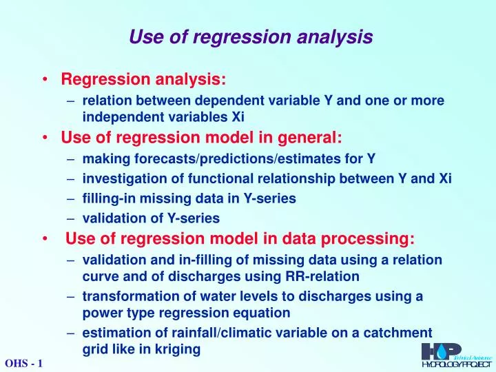
Use of regression analysis • Regression analysis: • relation between dependent variable Y and one or more independent variables Xi • Use of regression model in general: • making forecasts/predictions/estimates for Y • investigation of functional relationship between Y and Xi • filling-in missing data in Y-series • validation of Y-series • Use of regression model in data processing: • validation and in-filling of missing data using a relation curve and of discharges using RR-relation • transformation of water levels to discharges using a power type regression equation • estimation of rainfall/climatic variable on a catchment grid like in kriging OHS - 1
Linear and non-linear regression equations • Linear regression • simple linear regression (i = 1) • multiple and stepwise regression (i > 1) in stepwise-regression the independent variables enter model one by one based on largest reduction of unexplained variance (free variables); forced variables always enter model • Non-linear regression OHS - 2
Suitable regression model • Model depends on: • variables considered • physics of the processes • range of the data of interest • A non-linear relation may well be described by a linear regression equation within a particular range of the variables in regression • annual rainfall-runoff relation is in principle non-linear, but: • for low rainfall abstractions vary strongly due to evaporation • for very high rainfall evaporation has reached its potential and is almost constant • within a limited range relation assumption of linearity is often suitable OHS - 3
General form of relation between annual rainfall and runoff Evaporation Runoff = Rainfall OHS - 4
Use of regression model for discharge validation • Steps • develop regression model where runoff/discharge is regressed on rainfall: Qt = f(Pt, Pt-1,…..) • by investigating the time-wise behaviour of the residuals stationarity of the relationship is tested • if rainfall is error free deviations from stationarity may be due to: • change in drainage characteristics • incorrect runoff data due to errors in the water level data and/or in the stage-discharge relation • visualisation of non-stationarity by double mass analysis of observed discharge and via regression computed discharge OHS - 5
Simple linear regression model Ŷ = + X Residual = part of Y not explained by regression i Distribution of residuals Ŷi Ŷ = + X Y = + X + Y - Y = Y2 = Y2 + 2 Part of Y explained by regression Total variance = explained variance + unexplained variance OHS - 6
DIRECTION OF DATA VECTOR FOR REGRESSION ANALYSIS 3-D plot of monthly rainfall Direction for parameter estimation Years Months OHS - 7
Estimation of regression coefficients • Minimising the sum of squared errors to obtain Least Squares Estimators: • First derivatives of M to a and b set to zero: normal equations: • Solutions for b and a OHS - 8
Measure for goodness of fit • Other forms of regression equation (Y - Y) = b(X - X) • Or with correlation coefficient r = SXY/X.Y: (Y - Y) = r Y/X(X - X) • By squaring previous equation and averaging • 2 = Y2 (1 - r2) • r2 = coefficient determination • r2 is a measure for the quality of the regression fit • NOTE: A high r2 is not sufficient; behaviour of residual about regression line and development with time also extremely important OHS - 9
Confidence limits • Error variance • Confidence limits regression line • Confidence limits prediction MIND THE DIFFERENCE OHS - 10
Application of regression analysis for data validation • 17 years of annual rainfall and runoff data • Procedure: • Plotting of time series • Fitting of regression equation R = f(P) • Plot of residual versus P • Plot of residual versus time • Plot of accumulated residual with time • Double mass analysis of observed versus regression based runoff • Adjustment of runoff data • Repetition of above procedure and compare with above • Compare coefficients of determination • Compute confidence limits about regression and for prediction OHS - 11
Rainfall-runoff record 1961-1977 OHS - 12
Regression fit rainfall-runoff OHS - 13
Plot of residual versus rainfall OHS - 14
Plot of residual versus time OHS - 15
Plot of accumulated residual OHS - 16
Double mass analysis of observed versus computed runoff Break in measured runoff OHS - 17
Extrapolation Extrapolation of a regression equation beyond the measured range of X to obtain a value of Y not recommended: • confidence intervals become large • relation Y = f(X) may be non-linear for full range of X • extrapolation only if evidence of applicability of relation OHS - 23
Multiple linear regression models • Model for monthly rainfall: R(t) = + 1P(t) + 2P(t-1)+…. • General linear model Y = 1X1 + 2X2+….….+ pXp + • Matrix form: Y = X + where: Y = (nx1) - data vector of (yi-y) X= (nxp) - data matrix of (xi1-x1),…,(xip-xp) = (px1) - column vector of regression coeff. = (nx1) - column vector of residuals Centered about the mean OHS - 24
Estimation of regression coefficients • Minimisation of residual sum of squares T: T = (Y - X)T(Y - X) • Differentiating with respect to and replacing by its estimate b normal equations: XTXb = XTY • For b it follows: b = (XTX)-1XTY with: E[b] = Cov(b) = 2(XTX)-1 OHS - 25
Analysis of variance table (ANOVA) Total sum of squares about the mean = regression sum of squares + + residual sum of squares Coefficient of determination = Rm2 = SR/SY = 1 - Se/SY OHS - 26
Coefficient of determination From ANOVA table • Coefficient of determination Rm2 Rm2 = SR/SY = 1 - Se/SY • Coefficient of determination adjusted for number of independent variables in regression Rma2 Rma2 = 1 - MSe/MSY = 1 - (1 - Rm2).(n - 1)/(n - p - 1) OHS - 27
Comments • Points of concern in using multiple regression: • can a linear model be used • what independent variables should be included • Independent variables may be mutually correlated • investigate through the correlation matrix • Retaining variables in regression that are highly correlated complicate interpretation of regression coefficients, with physically nonsense values • Apply stepwise regression to select the “best” regression equation • In stepwise regression a distinction can be made between “free” and “forced” variables; May enter regression dependent on correlation Will enter regression irrespective of correlation OHS - 28
Non-linear models • By transformation non-linear models can be transformed to linear models, e.g. Y = X to: ln Y = ln + ln X or: YT = T + T XT where: YT = ln Y XT = ln X T = ln T = • Remarks: • The transformed residual sum of squares is minimised rather than the residual sum of squares • Error term is additive in the transformed state, i.e. multiplicative in the power model: T = ln OHS - 29
Filling-in missing data • Filling-in of missing water level and rainfall data in previous modules • Filling in of discharge data using regression relation with rainfall often suitable for monthly, seasonal or annual data • Monthly regression model e.g.: Qk,m = ak + b1kPk,m + b2kPk-1,m + se,k e • Addition of random component yes or no • Note: E[e] = 0, hence for single value no random component • For longer in-filling: could be considered dependent on use as no addition reduces the variance of series Regression model for month k, computing values for Q in year m OHS - 30
Type of regression model for filling-in missing flows • Previously the following rainfall-discharge relation was proposed: • Often regression coefficients do not vary much from month to month, but rather with wetness of month. Two sets of parameters are used in a regression model for all or a number of months: • one set for dry conditions • another set for wet conditions • In the latter approach the non-linear relationship is fitted by two linear models Qk,m = ak + b1kPk,m + b2kPk-1,m + se,k e OHS - 31