Decomposition Method

1. Decomposition Method

2. Types of Data • Time series data: a sequence of observations measured over time (usually at equally spaced intervals, e.g., weekly, monthly and annually). Examples of time series data include: Gross Domestic Product each quarter; annual rainfall; daily stock market index • Cross sectional data: data on one or more variables collected at the same point in time

3. Time Series vs Causal Modeling • Causal (regression) models: the investigator specifies some behavioural relationship and estimates the parameters using regression techniques; • Time series models: the investigator uses the past data of the target variable to forecast the present and future values of the variable

4. Time Series vs Causal Modeling • On the other hand, there are many cases when one cannot, or one prefers not to, build causal models: • insufficient information is known about the behavioural relationship; • lack of, or conflicting, theories; • insufficient data on explanatory variables; • expertise may be unavailable; • time series models may be more accurate

5. Time Series vs Causal Modeling • Direct benefits of using time series models: • Little storage capacity is needed; • some time series models are automatic in that user intervention is not required to update the forecasts each period; • some time series models are evolutionary in that the models adapt as new information is received;

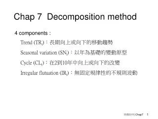
6. Classical Decomposition of Time Series • Trend – does not necessarily imply a monotonically increasing or decreasing series but simply a lack of constant mean, though in practice, we often use a linear or quadratic function to predict the trend; • Cycle – refers to patterns or waves in the data that are repeated after approximately equal intervals with approximately equal intensity. For example, some economists believe that “business cycles” repeat themselves every 4 or 5 years;

7. Classical Decomposition of Time Series • Seasonal – refers to a cycle of one year duration; • Random (irregular) – refers to the (unpredictable) variation not covered by the above

8. Decomposition Method • Multiplicative Models • Additive Models Find the estimates of these four components.

9. Multiplicative Decomposition • Examples: (1) US Retail and Food Services Sales from 1996 Q1 to 2008 Q1 (2) Quarterly Number of Visitor Arrivals in Hong Kong from 2002 Q1 to 2008 Q1 Figure 2.1 Figure 2.2

10. Figure 2.1 US Retail Sales Back

11. Figure 2.2 Visitor Arrivals

12. Cycles are often difficult to identify with a short time series. • Classical decomposition typically combines cycles and trend as one entity:

13. Illustration : Consider the following 4-year quarterly time series on sales volume:

14. Figure 2.3

15. Step 1 : Estimation of seasonal component (SNt) • Yt = TCt SNt  IRt • Moving Average for periods 1 – 4 Moving Average for periods 2 – 5

17. Assuming the average of the observations is also the median of the observations, the MA for periods 1 – 4, 2 – 5, 3 – 6 are centered at positions 2.5, 3.5 and 4.5 respectively.

18. To get an average centered at periods 3, 4, 5 etc. the means of two consecutive moving averages are calculated: Centered Moving Average for period 3 Centered Moving Average for period 4

20. Because the CMAtcontains no seasonality and irregularity, the seasonal component may be estimated by

22. After all have been computed, they are further averaged to eliminate irregularities in the series. We also adjust the seasonal indices so that they sum to the number of seasons in a year (i.e., 4 for quarterly data, 12 for monthly data). Why?)

23. Quarter Average 1 (0.628748707 + 0.6 + 0.588555858)/3=2 (0.894211577 + 0.911004785 + 0.949512843)/3=3 (0.989429175 + 1.013645224 + 0.970616114)/3=4 (1.445378151 + 1.499516908 + 1.49860205)/3= Sum =

24. Step 2 : Estimation of Trend/Cycle • Define deseasonalized (or seasonally adjusted) series as for example, D1 = 72/0.6063 = 118.7506

26. TCt may be estimated by regression using a linear trend: where b0 and b1 are least squares estimates of 0 and1 respectively.

27. EXCEL regression output :

28. For example,

30. Step 3 : Computation of fitted values and out-of-sample forecasts

31. Out of sample forecast :

33. Figure 2.4

34. Measuring Forecast Accuracy : 1) Mean Squared Error • Mean Absolute Deviation

35. Method AMethod B et = – 2 – 4 1.5 0.7 –1 0.5 2.1 1.4 0.7 0.1 Method A : MSE = 2.43 MAD = 1.46 Method B : MSE = 3.742 MAD = 1.34

36. Naive Prediction if U = 1  Forecasts produced are no better than naive forecast U = 0  Forecasts produced perfect fit The smaller the value of U, the better the forecasts. Theil’s u Statistics

37. MSE = 11.932 MAD = 2.892 Theil’s U = 0.0546

38. Out-of-Sample Forecasts • Expost forecast • Prediction for the period in which actual observations are available • Exante forecast • Prediction for the period in which actual observations are not available.

39. Ex-ante forecast Ex-post forecast in-sample simulation “back” casting T2 T1 T3 Time (today) estimation period

40. Additive Decomposition Yt Yt Trend Trend Time (Multiplicative Seasonality) (Additive Seasonality) Time

41. Multiplicative decomposition is used when the time series exhibits increasing or decreasing seasonal variation (Yt=TCt  SNt  IRt)

42. Additive decomposition is used when the time series exhibits constant seasonal variation (Yt=TCt + SNt + IRt)

43. Step 1 : Estimation of seasonal component (SNt) • Calculation of MAtand CMAt is the same as per multiplicative decomposition • Initial seasonal component may be estimated by For example,

44. Seasonal indices are averaged and adjusted so that they sum to zero (Why?)

46. Step 2 : Estimation of Trend/Cycle • Deseasonalized series is defined as • TCtmay be estimated by regression as per multiplicative decomposition

47. i.e., Dt = o + 1t + t and Multiplicative decomposition

48. So, and For example, and

49. MSE = 27.911 MAD = 4.477