Lead Time Dependent Product Deterioration in Manufacturing Systems: Constraints and Solutions

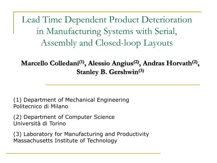
1. Lead Time Dependent Product Deterioration in Manufacturing Systems with Serial, Assembly and Closed-loop Layouts Marcello Colledani(1), AlessioAngius(2),Andras Horvath(2), Stanley B. Gershwin(3) (1) Department of Mechanical Engineering Politecnico di Milano (2) Department of Computer Science Università di Torino (3) Laboratory for Manufacturing and Productivity Massachusetts Institute of Technology

2. Full Empty Full Empty Full Empty Full Empty , Lead time constraints in manufacturing systems Lead time constraints in manufacturing systems are usually due to: Perishable or deteriorating products; Strict customer delivery requirements. • Perishable, or obsolete, or deteriorating products are allowed to spend a limited amount of time inside the manufacturing system (or a portion of system). • If the system flow time, or lead time, LT exceeds a certain fixed threshold the product has to be considered as a defect and has to be scrapped by the system. Finished products. Raw Material. • Challenges: • Machine unreliability. • Buffers sizes and production • control policies. Strong impact of the system dynamics on the product quality.

3. Industrial motivation – lead time constraints 1- Production of fresh food, such as yoghurt. • Strict requirements on hygiene. • A typical production sequence includes: • 1) mixing/standardizing of milk, • 2) pasteurization, • 3) fermentation, • 4) cooling, • 5) addition of fruit additives, • 6) packaging. • A typical daily order base is 500 000 units. • Maximum storage time before packaging, 2- Production of multi-layer, multi-lumen micro-catheters for medical applications. Additives • Challenges: • The lead time between the drying and extrusion processes should not exceed a certain limit to avoid increase of the moisture level by exposure to the air. • Excessive moisture level affects the material viscosity. • This results in fluctuations of the material shear rate and instability in the extrusion process, thus affecting the quality of the tube section. Rawmaterialcharacterization and treatment 3- Production of high-tech electronics products and semiconductor wafers (deterioration due to exposure to dust). 4- Production of drugs and medicines (deterioration due to temperature variations). 5- Body painting process in car body manufacturing (dust contamination by exposure to the air). (EU Project MuProD - Innovative proactive Quality Control system for in-process multi-stage defect reduction –FOF.NMP.2011.5: “Towards zero-defect manufacturing”) Raw parts Quality Correlation ELEMENTS ProcessStages M2: drying M3: compounding M4: extrusion M5: forming Inspection Stage M0: integrity test M1: moisture test Yoghurt production at Arla Foods, Sweden Die production by micro-milling, micro-EDM. Micro-catheters (Ø0.2mm – Ø3mm).

4. Literature review • Impact of system design on product quality (no perishable goods): • Colledani M., Fischer A., Iung B., Lanza G., Schmitt R., Tolio. T., Vancza J., Design and management of manufacturing systems for production quality, CIRP Annals - Manufacturing Technology, Volume 63, Issue 2, 2014. • R. R. Inman, D. E. Blumenfeld, N. Huang, and J. Li, Survey of recent advances on the interface between production system design and quality, IIE Transactions, vol. 45/6, pp. 557–574, 2013. • M. Colledani and T. Tolio, Integrated quality, production logistics and maintenance analysis of multi-stage asynchronous manufacturing systems with degrading machines, CIRP Annals-Manufacturing Technology, vol. 61/1, pp. 455–458, 2012. • Kim and S. Gershwin, Integrated quality and quantity modeling of a production line, OR spectrum, vol. 27/2, pp. 287–314, 2005. • Manufacturing of perishable products (no lead time analysis): • G. Liberopoulos, G. Kozanidis, and P. H. Tsarouhas, Performance evaluation of an automatic transfer line with WIP scrapping during long failures, Manufacturing and Service Operations, vol. 9/1, p. 6283, 2007. • Wang, Y. Hu, and J. Li, Transient analysis to design buffer capacity in dairy filling and packing production lines, Journal of Food Engineering, vol. 98/1, p. 112, 2010. • Part-release policies for lead time control (only Bernoulli lines): • Biller, S., Meerkov, S., and Yan, C.B. (2013). Raw material release rates to ensure desired production lead time in bernoulli serial lines. International Journal of Production Research, 51, 4349–4364. • Naebulharam, R., Zhang, L., 2014, Bernoulli Serial Lines with Deteriorating Product quality: Performance Evaluation and System‐theoretic Properties. International Journal of Production Research, 52/5: 1479‐1494. • Lead time analysis (only simple manufacturing system settings): • C. Shi and S. Gershwin, Part waiting time distribution in a two- machine line, in Proc. of the 14th IFAC Symposium on Information Control Problems in Manufacturing, 2012, pp. 457–462. • M. Colledani, Angius A., Horvath A. Lead Time Distribution in Unreliable Production Lines Processing Perishable Products, ETFA Emergin Technology and Factory Automation, Barcelona, Spain, 2014.

5. Objective and research strategy • To develop a methodology for modeling and analyzing the performance of manufacturing systems under lead time constraints. Finished products. Raw Material. • Research Strategy: • Derive the lead time distribution in unreliable manufacturing systems, under general system architecture and machines’ behavior. • Calculate the relevant performance measures for systems under lead time constraints (e.g. due to part quality deterioration). • Investigate the impact of the system parameters on the performance measures. • Derive system design and management rules.

6. Modelling Assumptions – System Architectures The system architecture can be described in form of a directed graph as the set W of connections between generic stages i and j. Fixed population Np of parts circulating in the system. For each machine Mj the input buffers is in the set Uj.

7. Modelling Assumptions – System Features • The flow of material in the system is discrete. • Each buffer Bi,j is located between machines Mi and Mj and has finite capacity denoted as Ni,j • Blocking Before Service (BBS) protocol is assumed.

8. Modelling Assumptions - Machines’ behavior We consider General Markovian Machines with multiple operational and down states ([Gershwin, Fallah-Fini, 2007], [Colledani 2011]). m=1 m=0 • Machine Mk is characterized by a set of states Sk, with dimensionality Ik. • A binary reward vector mkis considered with size Ik: • mkj=1, if Mk is operational in state j and processes one part per time unit; • mkj=0, if Mk is down in state j and it does not produce. • The operational states are in the set Uk and the down states are in the set Dk. • The machine dynamics is regulated by the transition probability matrix lk (Ik Ik matrix). • Transitions are Operation Dependent.

9. Assumptions – Lead Time dependent deterioration LT LT Critical portion of the system:is composed of those buffers that are between stages Me and Mq, in the direction of the material flow. Quality deterioration function g(h): probability that a part released by the system is defective given that it spent h time units in the critical portion of system.

10. Performance Measures • The average total production rate of the system, ETot, calculated neglecting the lead time constraint; • The probability that the lead time LT is equal to the number of time units, h, i.e. P(LT=h); • Theaverage effective production rate, Eeff, only considering parts that respect the lead time constraint. It is given by: • The system yield, YSystem, i.e. the fraction of products respecting the lead time constraint; • The average Work in Progress, WIP, total average inventory in the system.

11. Calculation of the lead time distribution – simple example • The dynamics of the system in visiting its states s=(n1,2,a1,a2) can be modeled as a DTMC with transition probability matrix R. • The steady state probability vector is denoted as p. • Where: • pE (b,a2): the probability that, when the part enters the buffer, it is in position b and Machine 2 is in state a2. • qa2(h,b): the probability that a part leaves the system in h time units given that it enters the buffer in position b and the second machine is in state a2. P(LT=h) b Machine 1 Machine 2

12. Calculation of the lead time distribution – simple example (N1,2,D) (N1,2-1,U) (N1,2-1,D) (2,U) (2,D) The LT is the time to absorption of a MC with initial state (b,a2), final state (0,U) and transition matrix RT. (1,U) (1,D) 1-r2 (0,U) r2 1-r2 p2 1-p2 • RE: matrix which contains only those transition probabilities of R that correspond to placing a part in the buffer. 1-r2 p2 r2 1-p2 1-r2 p2 r2 1-p2

13. Calculation of the lead time distribution – Arbitrarily long serial and assembly line s=(a1,.., aK,n1,2,.., nK-1,K), R, p, RE, pE Critical portion s’=(ae+1,.., aK,ne,e+1,.., nK-1,K), RT, pT • Denote by pT,h the transient probabilities after h steps: • The lead time distribution is:

14. , , Calculation of the lead time distribution – loop systems Critical Portion Np=19 Critical Portion • There is need to classify the pallets in the critical portion of system: • “Inner” pallets: those that are already in the critical portion of system when the part enters it. • “Outer” pallets: the remaining parts. • Inner pallets become outer pallets when the leave the critical portion of the system.

15. , Calculation of the lead time distribution – loop systems • s=(a1,.., aK,n1,2,.., nK,1), R, p, RE, pE Critical Portion • s’=(a1,.., aK,b1,2,.., bK,1,c1,2,..,cK,1), RT, pT • bi,j: number of “outer” pallets in Bi,j • ci,j: number of “inner” pallets in Bi,j • The lead time distribution is:

16. , Effect on the Lead Time Distribution LT • Identical up-down machines. p=0.01, r=0.1. Identical buffers, N=5. e=1,q=5. The lead time distribution is multimodal, with a number of peaks equal to the number of stages K. The j-th peak, with j=1,..,q-e+1, is found for a number of time units given by this equation. If e=1, q=K

17. , Impact of the Buffer Size LT • Identical up-down machines. p=0.01, r=0.1. Identical buffers, N=5. e=1,q=5. h*=35

18. Analysis of Assembly Systems LT • Identical up-down machines. p=0.01, r=0.1. Identical buffers, N=5. e=1,q=5. h*=35 Lead time for the 6 machine assembly line. Lead time for the serial line, with 5 machines.

19. Analysis of Loop Systems LT • Identical up-down machines. p=0.01, r=0.1. Identical buffers, N=5. e=1,q=5. h*=35 • The effective throughput of CONWIP is higher that of the serial line.

20. Conclusions • Major findings: • Calculation of the lead time distribution in general system architectures and machines’ behavior. • Derivation of the main performance measures, under lead time constraints imposed by product deterioration. • Insights on the system behavior gathered from numerical results. • Future Research: • Extension to longer systems through decomposition and propagation of lead time distributions. • Application to multiple loops. • Application to other areas (e.g. supply chain management, production planning).

21. Lead Time Dependent Product Deterioration in Manufacturing Systems with Serial, Assembly and Closed-loop Layouts Marcello Colledani(1), AlessioAngius(2),Andras Horvath(2), Stanley B. Gershwin(3) (1) Department of Mechanical Engineering Politecnico di Milano (2) Department of Computer Science Università di Torino (3) Laboratory for Manufacturing and Productivity Massachusetts Institute of Technology

22. , Effect on the Lead Time Distribution • Identical up-down machines. p=0.01, r=0.1. Identical buffers, N=10. e=1,q=5. • Identical up-down machines. p=0.05, r=0.5. Identical buffers, N=10. e=1,q=5.

23. B1,2 Impact of the Buffer Size M1 M2 h*=40 1- What is the motivation? 2- What is the reason for the discontinuity? 3- For what buffer size is it observed? It does not make sense to have a buffer size larger than h*+1.

24. , Effect on the Line Length • Identical up-down machines. p=0.01, r=0.1. Identical buffers, N=10. e=1,q=5.