Download
1 / 22
240 likes | 291 Views
Measures of Central Tendency:. Outline of the Course. III . Descriptive Statistics A . Measures of Central Tendency (Chapter 3) 1 . Mean 2 . Median 3 . Mode B . Measures of Variability (Chapter 4) 1 . Range 2 . Mean deviation 3 . Variance 4 . Standard Deviation

E N D
Outline of the Course III. Descriptive Statistics A. Measures of Central Tendency (Chapter 3) 1. Mean 2. Median 3. Mode B. Measures of Variability (Chapter 4) 1. Range 2. Mean deviation 3. Variance 4. Standard Deviation C. Skewness (Chapter 2) 1. Positive skew 2. Normal distribution 3. Negative skew D. Kurtosis 1. Platykurtic 2. Mesokurtic 3. Leptokurtic
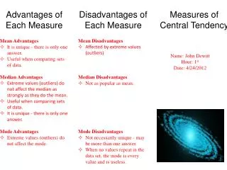
Measures of Central Tendency • The goal of measures of central tendency is to come up with the one single number that best describes a distribution of scores. • Lets us know if the distribution of scores tends to be composed of high scores or low scores.
Measures of Central Tendency • There are three basic measures of central tendency, and choosing one over another depends on two different things. • 1. The scale of measurement used, so that a summary makes sense given the nature of the scores. • 2. The shape of the frequency distribution, so that the measure accurately summarizes the distribution.
Measures of Central TendencyMode • The most common observation in a group of scores. • Distributions can be unimodal, bimodal, or multimodal. • If the data is categorical (measured on the nominal scale) then only the mode can be calculated. • The most frequently occurring score (mode) is Vanilla.
Measures of Central TendencyMode • The mode can also be calculated with ordinal and higher data, but it often is not appropriate. • If other measures can be calculated, the mode would never be the first choice! • 7, 7, 7, 20, 23, 23, 24, 25, 26 has a mode of 7, but obviously it doesn’t make much sense.
Measures of Central TendencyMedian • The number that divides a distribution of scores exactly in half. • The median is the same as the 50th percentile. • Better than mode because only one score can be median and the median will usually be around where most scores fall. • If data are perfectly normal, the mode is the median. • The median is computed when data are ordinal scale or when they are highly skewed.
Measures of Central TendencyMedian • There are three methods for computing the median, depending on the distribution of scores. • First, if you have an odd number of scores pick the middle score. • 1 4 6 7 12 14 18 • Median is 7 • Second, if you have an even number of scores, take the average of the middle two. • 1 4 6 7 8 12 14 16 • Median is (7+8)/2 = 7.5 • Third, if you have several scores with the same value in the middle of the distribution use the formula for percentiles (not found in your book).
Measures of Central TendencyMean • The arithmetic average, computed simply by adding together all scores and dividing by the number of scores. • It uses information from every single score. • For a population: For a Sample:
Measures of Central TendencyMeanOther Notes • If data are perfectly normal, then the mean, median and mode are exactly the same. • I would prefer to use the mean whenever possible since it uses information from EVERY score. • Though the preferred symbol for the mean is an X with a line over the top, creating this symbol is pretty tricky on the computer. APA style says:
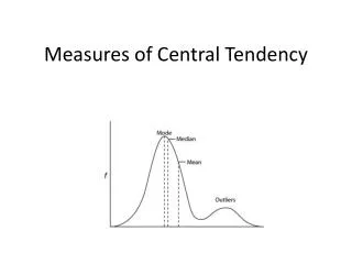
Measures of Central TendencyThe Shape of Distributions • With perfectly bell shaped distributions, the mean, median, and mode are identical. • With positively skewed data, the mode is lowest, followed by the median and mean. • With negatively skewed data, the mean is lowest, followed by the median and mode.
Measures of Central TendencyMean vs. MedianSalary Example • On one block, the income from the families are (in thousands of dollars) 40, 42, 41, 45, 38, 40, 42, 500 • SX=788, • The Mean salary for this sample is $98,500 which is more than twice almost all of the scores. • Arrange the scores 38, 40, 40, 41, 42, 42, 45, 500 • The middle two #’s are 41 and 42, thus the average is $41500, perhaps a more accurate measure of central tendency.
Measures of Central TendencyMean vs. MedianReaction Time Example • Data is time to complete task (in s): • 45, 34, 87, 56, 21, didn’t finish, 49 • It is not possible to compute a mean with this unknown number. • Even though we do not know this person’s time, I do know it is REALLY big. • 21, 34, 45, 49, 56, 87, something bigger • The median is the middle number, 49
Measures of Central TendencyMeanAlgebra Revisited • Its useful to consider the formula as the same as any other algebraic formulas, subject to the same rules. • Therefore, if we know the mean of a group of scores, we can figure out the SX.
Measures of Central TendencyMeanWeighted Mean • Lets pretend that one semesters class of 23 students scored M1 = 18 points on a quiz. The same quiz was then given the next semester to 34 students who then got M2 = 22 points. What is the overall (weighted) mean for these 57 students. • SX1 can be computed by multiplying M1 times the sample size (SX1= M1*n1 = 18*23 = 414). • For the second class, SX2 = M2*n2 = 22 * 34 = 748 • SXtotal = SX1 + SX2 = 414 + 748 = 1206 • ntotal = n1 + n2 = 23 + 34 = 57 • Mtotal = SXtotal / ntotal = 1206/57 = 21.158
Measures of Central TendencyMeanAdding a Score • On the first exam, 15 students had M = 85. • One kid came in late and took the test and scored 53, what is Mnew? • SXoriginal = Moriginal*noriginal = 85*15 = 1275 • SXnew = SXoriginal + new score = 1275 + 53 = 1328 • nnew = noriginal + 1 • Mnew = SXnew/nnew = 1328/16 = 83
Measures of Central TendencyMeanChanging an Existing Score • On the first exam, 16 students had M = 83. • One kid came in after the test and complained, I listened and decided to give him 10 extra points, now what? • SXoriginal = Moriginal*noriginal = 83*16 = 1328 • SXnew = SXoriginal + extra points = 1328 + 10 = 1338 • Mnew = SXnew/n = 1338/16 = 83.625
Measures of Central TendencyMeanTransformations • If a constant is added (or subtracted) to each score, the same constant will be added (or subtracted) to the mean. • If M for an exam is 82, then I find that I screwed up a question and give everyone 5 extra points, M simply becomes 82+5=87. • If every score is multiplied or divided by a constant number, then the mean will also be multiplied or divided by the same number. • This last property is particularly useful when converting between units of measurement. • If the M for the height of a group of first-graders is 47 inches, but I need to know their heights in cm I could: • Take every kids height * 2.54, then recompute M • Or, I could take the mean times 2.54 and conclude the M height of these kids is 119.38 cm.
Measures of Central TendencyDeviations around the Mean Exam Score • A common formula we will be working with extensively is the deviation: SX = 72 n = 8
Measures of Central TendencyUsing the Mean to Interpret DataPredicting Scores • If asked to predict a score, and you know nothing else, then predict the mean. • However, we will probably be wrong, and our error will equal: • A score’s deviation indicates the amount of error we have when using the mean to predict an individual score.
Measures of Central TendencyUsing the Mean to Interpret DataDescribing a Score’s Location • If you take a test and get a score of 45, the 45 means nothing in and of itself. However, if you learn that the M = 50, then we know more. Your score was 5 units BELOW M. • Positive deviations are above M. • Negatives deviations are below M. • Large deviations indicate a score far from M. • Large deviations occur less frequently.
Measures of Central TendencyUsing the Mean to Interpret DataDescribing the Population Mean • Remember, we usually want to know population parameters, but populations are too large. • So, we use the sample mean to estimate the population mean.