Download

1 / 0
0 likes | 170 Views
Two questions occurred to me on first seeing this diagram which incidentally is taken from: Fluid Mechanics Fundamentals and Applications Y. A. Cengel and J. M. Cimbala . McGraw Hill.

E N D