Download
1 / 39
390 likes | 394 Views
This study evaluates the performance of different NWP ensemble configurations for atmospheric transport and dispersion (AT&D) applications. The use of ensembles provides a better estimate of atmospheric variability, improving AT&D forecasts. The study includes down-selection of ensemble members using Principal Component Analysis (PCA) weighting and post-processing using Bayesian Model Averaging (BMA).

E N D
Evaluating NWP Ensemble Configurations for AT&D Applications Jared A. Lee1,2, Walter C. Kolczynski1, Tyler C. McCandless1,2, Kerrie J. Long2, Sue Ellen Haupt1,2, David R. Stauffer1, and Aijun Deng1 The Pennsylvania State University1Department of Meteorology2Applied Research Lab University Park, PA21 January 201016th Conference on Air Pollution 90th AMS Annual Meeting - Atlanta, GA 12.3
Why Use Ensembles? • Single deterministic forecasts could be outliers in the forecast probability density function (PDF) • NWP ensembles provide a better estimate of the atmospheric variability in a given situation by approximating the PDF of the atmospheric state • Grimit and Mass (2002) - WAF: Correlation exists between ensemble spread and forecast uncertainty • NWP ensemble uncertainty information can improve AT&D forecasts [e.g., Lee et al. (2009) - JAMC] Four MREF members on Penn State e-Wall
Sources of Uncertainty • Many atmospheric transport & dispersion (AT&D) models are driven by numerical weather prediction (NWP) model output • Uncertainty estimates for concentration predictions by AT&D models must account for both AT&D and NWP model uncertainty • Many sources of uncertainty in NWP models • Initial conditions (ICs) • Lateral/lower boundary conditions (LBCs) • Model physics parameterizations • Numerics Initial Conditions (ICs) Lateral Boundary Conditions (LBCs) NWP Model AT&D Model Model Physics Parameterizations
WRF-ARW v3.1.1 36-km domain, no nests 45 vertical levels GFS 0.5° ICs/LBCs 18-member physics (PH) ensemble 48-h forecasts starting at 00 UTC daily (12 UTC in the future as well) 04–17 Jan 2009 Winter Evaluation Period • Different synoptic regimes in both weeks: • 04-10 Jan: Deep, digging trough moving across U.S. • 11-17 Jan: Persistent ridge in west & trough in east • Important to evaluate performance of ensemble members in a range of regimes
Why Down-select? • We want to include other sources of variability in addition to physics options, including IC/LBC and/or multi-model uncertainty • We know that IC/LBC and PH variability sample different parts of the forecast PDF • Fujita et al. (2007) – MWR: • IC variability – spread in dynamic variables (u,v) • PH variability – spread in thermodynamic variables (θ,q) • Potential way to do this: select a small number of physics runs as “control” members around which to perturb the ICs/LBCs using an EnKF (from DART) • e.g., 5 ctrl * 5 pert = 25 members • We lack computational resources to run large numbers (dozens) of ensemble members • We want to create a long-term stable NWP ensemble dataset for AT&D research
Ensemble Down-SelectionPrincipal Component Analysis (PCA) PCA Weighting -Principal Component Analysis is a mathematical procedure that transforms a number of possibly correlated variables (ensemble members, in this case) into a smaller number of uncorrelated variables called principal components -The first principal component accounts for as much variability in the data as possible -Uses the factors (how much each ensemble member contributed) from the first principal components -The factors from the first principal component are the ensemble member weights Credit: Tyler McCandless
Ensemble Down-SelectionPCA Weighting Results • The selection of ensemble members appears directly related to the parameter being forecast • 2-m Temperature: No member using Thermal Diffusion land surface scheme (1,2,7,8,13,14) was selected at any forecast lead time • 10-m Wind Speed: Members that were selected varied somewhat by parameter (u-wind, v-wind) and forecast lead time (24h, 36h, 48h) • Ensemble members 3,4,10,11,12 were always selected • Varying the cumulus scheme appears to have had almost no effect during this time period • PCA Weighting evaluates the deterministic predictive ability of the ensemble, while other methods examine both the deterministic and probabilistic predictive ability of the ensemble Credit: Tyler McCandless
Post-ProcessingBayesian Model Averaging (BMA) • Bayesian Model Averaging (BMA) main tool for calibration in this study • Assumes a normally distributed conditional probability around each ensemble member • Estimates the optimal weights and standard deviations using expectation-maximization • Also use correlation to identify impact of different parameterizations and possible redundancy Credit: Walter Kolczynski
Post-ProcessingBMA Demonstration Legend: Blue Conditional probability for individual member Red Cumulative probability for full ensemble Black Observed temperature p(T) dT Temperature (K) Credit: Walter Kolczynski
Post-ProcessingBMA Weights Thermal Diffusion Land Surface Model Credit: Walter Kolczynski
Post-ProcessingBMA Weights Noah Land Surface Model Credit: Walter Kolczynski
Post-ProcessingBMA Weights RUC Land Surface Model Credit: Walter Kolczynski
Post-ProcessingBMA Weights ACM2 PBL & Pleim-Xu Sfc Credit: Walter Kolczynski
Post-ProcessingMember Correlations for 2-m Temp 2-m T correlation Credit: Walter Kolczynski
Post-ProcessingMember Correlations for 10-m U-wind 10-m U correlation Credit: Walter Kolczynski
06 Jan 2009 00z – YSU PBLSCIPUFF 36-h Continuous Releases Thermal Diff. mem01 mem02 Noah mem03 mem04 RUC mem05 mem06
06 Jan 2009 00z – MYJ PBLSCIPUFF 36-h Continuous Releases Thermal Diff. mem07 mem08 Noah mem09 mem10 RUC mem11 mem12
06 Jan 2009 00z – ACM2 PBLSCIPUFF 36-h Continuous Releases Thermal Diff. mem13 mem14 Noah mem15 mem16 RUC mem17 mem18
18 Jan 2009 00z – YSU PBLSCIPUFF 36-h Continuous Releases Thermal Diff. mem02 mem01 Noah mem03 mem04 RUC mem05 mem06
18 Jan 2009 00z – MYJ PBLSCIPUFF 36-h Continuous Releases Thermal Diff. mem07 mem08 Noah mem09 mem10 RUC mem11 mem12
18 Jan 2009 00z – ACM2 PBLSCIPUFF 36-h Continuous Releases Thermal Diff. mem13 mem14 Noah mem15 mem16 RUC mem17 mem18
ConclusionsWinter Evaluation Period PH Ensemble Changes to the cumulus parameterization have little effect on the ensemble predictions for surface variables All methods of investigation show that the Thermal Diffusion Land Surface Model performs far poorer than the others for 2-m temperature BMA weights and ensemble member correlations indicate the PBL/Surface Layer scheme as dominant for 10-m winds (of those parameters varied)
Future Work Examine additional combinations of physics parameterizations Investigate performance of ensemble for additional evaluation periods and initial forecast times Create an ensemble that also perturbs initial conditions and boundary conditions Adjust the sensitivity of the PCA Weight Guided Feature Selection to determine the optimal number of ensemble members Find BMA weights for vector winds, not just components, and compute CRPS & RMSE for verification Find & compare results using a random 10 of 14 days for PCA & BMA methods
Supplementary Slides
Year-Long Ensemble • ~20 WRF members, run for 1 year • 2 cycles daily, 48 h starting at 00 & 12 UTC • Use ensemble data to drive SCIPUFF case studies • Very few regional scale field experiments • Create “truth” using SCIPUFF driven by a higher-resolution NWP dynamic analysis, as in Kolczynski et al. (2009) • Compute meteorological statistics for several ABL parameters (e.g., wind direction, temperature) • Compare performance of this ensemble to an existing ensemble (e.g., NCEP SREF)
Why Is This Important? • Most current short-range ensembles built for spread in QPF, like NCEP SREF, and not AT&D • No current agreement on best way to configure an NWP ensemble for AT&D forecasting • This will provide a long-term, consistent, short-range ensemble dataset for research purposes, particularly for the connection between meteorological and dispersion uncertainty • Potential to be the basis for an operational NWP ensemble configuration used by DTRA for emergency response after hazardous chem/bio releases
WRF-ARW Physics SchemesMicrophysics & Cumulus schemes • WSM 5-class microphysics scheme • Vapor, rain, snow, cloud ice, cloud water • Kain-Fritsch cumulus scheme • Moist updrafts & downdrafts, with entrainment & detrainment effects and simple microphysics • Grell-Devenyi cumulus scheme • An ensemble of 144 cumulus schemes are run in every grid box, the average is fed back to model • Differing entrainment/detrainment parameters, precipitation efficiencies, dynamic control closures to determine cloud mass flux
WRF-ARW Physics SchemesLand surface models (LSMs) • Thermal Diffusion LSM • 5-layer soil temperature model, 31cm depth • Soil moisture constant with land use type and season • No explicit vegetation effects • Noah LSM • 4-layer soil temperature and moisture model, 2m depth • Includes canopy moisture, fractional snow cover, soil ice • Explicit vegetation effects (incl. evapotranspiration, runoff) • Rapid Update Cycle (RUC) LSM • 6-layer soil temperature and moisture model, 5.25m depth • Multi-layer snow model • Includes vegetation effects and canopy water • Layer approach to solving moisture & energy budgets
WRF-ARW Physics SchemesSurface layer schemes • MM5 Similarity • Stability functions compute heat, moisture & momentum surface exchange coefficients • No thermal roughness length parameterization • Eta Similarity • Based on Monin-Obukhov similarity theory • Includes viscous sub-layer parameterizations • Surface fluxes computed iteratively • Pleim-Xu • Based on similarity theory • Includes viscous sub-layer parameterizations • Similarity functions estimated from analytical approximations from state variables
WRF-ARW Physics SchemesAtmospheric boundary layer (ABL) schemes • Yonsei University (YSU) • Critical bulk Richardson number (0.0) defines ABL top • Entrainment proportional to surface buoyancy flux • Mellor-Yamada-Janjić (MYJ) • Critical TKE value defines ABL top • Level 2.5 turbulence closure • Asymmetrical Convective Model v2 (ACM2) • Thermal profile defines ABL top • Combined local and non-local closure in convective boundary layer (CBL), eddy diffusion in stable boundary layer (SBL)