Ch 7: Analog pulse modulation

1. Ch 7: Analog pulse modulation

2. Final Exam Announcements • Final Exam • 다음주 수요일( 6월9일), 7~8교시(15:00-16:30) • In class • Open book and notes Jasnet 설명회: 6/3(목) 3:00~5:00

3. Types ofSignalTransmission

4. Digital Baseband Transmission

5. Digital Baseband Transmission

6. Analog – Digital 변환

7. Sampling (교과서 section 1.13) • Nyquist showed that it is possible to reconstruct a band-limited signal from periodic samples, as long as the sampling rate is at least twice the frequency of the of highest frequency component of the signal • Several types of sampling are available for pulse modulation Flat-Top Sampling (평탄 상단 표본화) Natural Sampling

8. Aperture Effect (개구효과) • 표본화 오차는 고주파 부분의 손실에 해당하는 것을 말함. Curve 에서 Flat-Top으로 (고차함수에서 저차함수로)

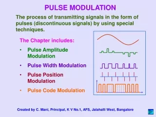
9. Sampling • Sampling alone is not a digital technique • The immediate result of sampling is a pulse-amplitude modulation (PAM) signal • PAM is an analog scheme in which the amplitude of the pulse is proportional to the amplitude of the signal at the instant of sampling • Another analog pulse-forming technique is known as pulse-duration modulation (PDM). This is also known as pulse-width modulation (PWM)

10. Analog Pulse-Modulation Techniques PAM PDM PPM

11. Sampling circuit with and without sample hold. Sample and hold will be used for pulse code Modulation

12. Rect and Sinc (교과서 예제 1.9) AT A -1/T -.5T .5T 1/T t 2/T f A/B A -.5B .5B f -1/B 1/B 2/B t

13. Sampling • Sampling (Time): • Sampling (Frequency) = x(t) nd(t-nTs) xs(t) 0 0 0 Xs(f) = X(f) nd(t-n/Ts) * -1/Ts 1/Ts 0 0 0 1/Ts

14. xp(t) x(t)d(t-(-T0)) x(t)d(t-2T0) x(t)d(t) x(t)d(t+2T0) x(t)d(t-T0) -T0 T0 -2T0 2T0 Xp(f)=X(f)(1/T0)Snd(f-n/T0)=Sn (1/T0)X(n/T0)d(f-n/T0) C0=f0X(0) Xp(f) c-1 c1=f0X(f0) f0 -f0 2f0 Fourier Transforms for Periodic Signals (교과서 1.12 주기적 시간함수) xp(t)=x(t)Snd(t-nT0)=nx(t)d(t-nT0) =ncnej2pn/T0 x(t) t 0 =ncnd(f-n/T0) X(f) f0=1/T0 f 0

15. X(f) Nyquist Sampling Theorem • A bandlimited signal [-B,B] is completely described by samples every Ts<.5/B secs. • Nyquist rate is 2B samples/sec • Recreate signal from its samples by using a low pass filter in the frequency domain Xs(f) X(f) -B 1/Ts>2B B .5/Ts -B B -1/Ts

16. Sampling in Frequency • By duality, can recover time limited signal by sampling sufficiently fast in frequency • Sampling in frequency is periodic repetition in time • Recover time limited signal by windowing Xs(f) x(t) xs(t) X(f) Fs=1/Ts t -.5Ts -Ts 0 Ts .5Ts f 0

17. Signal Recovery and Interpolation • Recover signal in frequency domain by passing sampled signal through LPF (rect) • In time domain this becomes convolution of samples with sinc function • Sinc function tracks signal changes between samples

18. Nyquistfrequency fs >2fm • Use a low Pass filter called a anti-aliasing before the sample and hold circuit to limit input freq of signal • Make sure that the sampling frequency rate(fs) is 2 times the sampled input signal frequency fs >2fm fs=1/Ts , B= fm

19. X´(f) Aliasing fs=1/Ts , B= fm • Aliasing occurs when a signal is sampled below its Nyquist rate • Repetitions in frequency domain overlap • Distortion (aliasing) in frequency domain Xs(f) X(f) -B -1/Ts B 1/Ts<2B B -B

20. - Fs 0 Fs 2Fs AliasingSpectrum of a pulsed signal fs >2fm - Fs 0 Fs 2Fs fs <2fm

21. Intersymbol Interference파형과부호간의 간섭 • Intersymbol Interference (ISI) • Eye Diagrams • Raised Cosine Filtering • Timing Recovery • Matched Filtering • Bit Error Rate (BER)

22. Intersymbol Interference …1 • With any practical channel the inevitable filtering effect will cause a spreading (or smearing out) of individual data symbols passing through a channel.

23. Intersymbol Interference …2 • For consecutive symbols this spreading causes part of the symbol energy to overlap with neighbouring symbols causing intersymbol interference (ISI).

24. Intersymbol Interference …3 • ISI can significantly degrade the ability of the data detector to differentiate a current symbol from the diffused energy of the adjacent symbols. • With no noise present in the channel this leads to the detection of errors known as the irreducible error rate.

25. Pulse Shape for Zero ISI부호간의 간섭이 0 이 되게 하는 파형 • Control the intersymbol interference such that it does not degrade the bit error rate performance of the link. • Achieved by ensuring the overall channel filter transfer function has what is termed a Nyquist frequency response (Nyquist 파형 ).

26. Nyquist Channel Response • transfer function has a transition band between passband and stopband that is symmetrical about a frequency equal to 0.5 x 1/ Ts. (minimum passband)

27. Nyquist Channel …2 • For such a channel the the data signals are still smeared but the waveform passes through zero at multiples of the symbol period.

28. Nyquist Channel …3 • If we sample the symbol stream at the precise point where the ISI goes through zero, spread energy from adjacent symbols will not affect the value of the current symbol at that point. • Inaccuracy in symbol timing is referred to as timing jitter.(타이밍의 부정확에 따른 지터)

29. Eye Diagrams • Visual method of diagnosing problems with data systems. • Generated using a conventional oscilloscope connected to the demodulated filtered symbol stream. • Oscilloscope is re-triggered at every symbol period or multiple of symbol periods using a timing recovery signal.

30. Eye Diagrams …2 • Resulting display is an ‘overlay’ of consecutive received symbol samples.

31. Eye Diagrams …3 • Example eye diagrams for different distortions, each has a distinctive effect on the appearance of the ‘eye opening’:

32. Raised Cosine Filtering • Commonly used realisation of a Nyquist filter. The transition band (zone between pass- and stopband) is shaped like a cosine wave.

33. Raised Cosine Filtering …2 • The sharpness of the filter is controlled by the parameter a, the filter roll-off factor. When a = 0 this conforms to the ideal brick-wall filter. • The bandwidth B occupied by a raised cosine filtered data signal is thus increased from its minimum value, Bmin = 0.5 x 1/Ts, to: • Actual bandwidth B = Bmin ( 1 + a)

34. Raised Cosine Transfer Function • 0.5{1 + cos[p(|f| - f1)/2fD]} — transition band

35. Impulse Response of Filter • The impulse response of the raised cosine filter is a measure of its spreading effect. • The amount of ‘ringing’ depends on the choice of a. • The smaller the value of a (nearer to a ‘brick wall’ filter), the more pronounced the ringing. • Note the next figure (taken from Couch p 185)uses the parameter ‘r’ rather than a.

36. Impulse Response of Filter …2

37. Choice of Filter Roll-off a • Benefits of small a • maximum bandwidth efficiency is achieved • Benefits of large a • simpler filter with fewer stages hence easier to implement • less signal overshoot • less sensitivity to symbol timing accuracy

38. Symbol Timing Recovery • Most symbol timing recovery systems obtain their information from the incoming message data using ‘zero crossing’ information in the baseband signal.