Download
1 / 56
570 likes | 816 Views
Chapter 2 Sampling and Construction. New Words. Contents. 2.1 Types of Signals in CCS 2.2 Sampling Process and Its Mathematical Description 2.3 Sampling Theorem and Some Problems 2.4 Reconstruction 2.5 Selection of Sampling Rate 2.6 Summarization. Clock. S/H &A/D. Computer. D/A.

E N D
Chapter 2 Sampling and Construction
Contents 2.1 Types of Signals in CCS 2.2 Sampling Process and Its Mathematical Description 2.3 Sampling Theorem and Some Problems 2.4 Reconstruction 2.5 Selection of Sampling Rate 2.6 Summarization
Clock S/H &A/D Computer D/A Holder Process Sensor 2.1 Types of Signals in CCS • A schematic diagram of a CCS is given in Figure 2.1. Figure 2.1: Schematic diagram of a CCS
2.1 Types of Signals in CCS • System signals can be classified as • According to time • According to the magnitude of the signal continuous time signal discrete time signal analog signal discrete signal digital signal
Digital signal Analog signal S/H Quantization Coding D A B C 2.1 Types of Signals in CCS • A-D converter: to convert continuous analog signal to digital signal Sample-and-hold circuit A-D converter Quantization Coding
2.1 Types of Signals in CCS Figure 2.2 A-D converter
Analog signal Digital signal Decoding Holder H G F 2.1 Types of Signals in CCS • D-A converter: to convert digital signal to continuous analog signal Decoding D-A converter Hold circuit
2.1 Types of Signals in CCS Fig. 2.3 Computer-controlled system • Types of the signals in a CCS • Analog signal (continuous in time and magnitude, such as signal A, H); • Digital signal (discrete in time and binary coding in magnitude, such as signal C, D, F, G); • Sampled signal (discrete in time and continuous in magnitude, such as signal B)
2.1 Types of Signals in CCS • Simplification of the two converters • Coding and decoding only change the formation of the signal, and they can be seen as equivalent transformation without error. • In general, quantization unit q is very small. We can ignore the effect aroused by it. • When hold time p in SHC circuit is insignificant with respect to the sample period of the control or with respect to the rate of change of the signal being sampled, the SHC is often seen as an ideal sampler. Figure 2.4 Simplification of Figure 2.3
p p t T T t T t 2.2 Sampling Process and Its Mathematical Description 2.2.1 Description of the sampling process Sampling period: T (s); Sampling frequency: f=1/T Hz Sampling angle frequency: rad/s Sampling process is unavoidable in computer-controlled systems.
1 t 0 1 t0 t 2.2 Sampling Process and Its Mathematical Description 2.2.2 Time domain description for ideal sampler and ideal sampled signal (1) Definition of Dirac function (2) Dirac function at t=t0
2.2 Sampling Process and Its Mathematical Description (3) An important property of Dirac function
1 -2T -T 0 T 2T t 2.2 Sampling Process and Its Mathematical Description (4) Description of the ideal sampler
2.2 Sampling Process and Its Mathematical Description (5) Time domain description of the ideal sampled signal • Let the input of the ideal sampler be x(t), the output of the ideal sampler is the ideal sampled signal x*(t) • In practice, we have x(t)=0 for t < 0, then the signal after the sampler can be expressed as (2.1)
1 2.2 Sampling Process and Its Mathematical Description where T(t) is the periodic function. And Eq. (2.1) is the time domain description of the ideal sampled signal and its diagram is shown in Fig. 2.7.
2.2 Sampling Process and Its Mathematical Description 2.2.3 Frequency domain description for ideal sampled signal (1) Fourier series
2.2 Sampling Process and Its Mathematical Description (2) Fourier transform As T approaches infinity, we define Frequency domain description of the ideal sampled signal
2.2 Sampling Process and Its Mathematical Description • When k = 0, • When k 0, X*(j) is periodic with s • when s > 2 max see Fig. 2.8(b) • when s = 2 max see Fig.2.8(c) • when s < 2 max see Fig.2.8(d)
2.2 Sampling Process and Its Mathematical Description • Nyquist frequency N = s/2 = /h (rad/sec) Example:
2.2 Sampling Process and Its Mathematical Description 2.2.4 Laplace Transform of sampled signal
2.2 Sampling Process and Its Mathematical Description • Relationship between X*(s) and X(s)
1 0 p -T -T+p T T+p 2.2 Sampling Process and Its Mathematical Description 2.2.5 Time domain description of real sampled signal
2.2 Sampling Process and Its Mathematical Description • The real sampled signal can be expressed as • If p<<T and the time constant of the input signal f(t), f*(t) can be approximated by
2.2 Sampling Process and Its Mathematical Description The Laplace transformations of the both sides of the above equation
2.2 Sampling Process and Its Mathematical Description 2.2.6 Frequency domain description of real sampled signal
2.2 Sampling Process and Its Mathematical Description 2.2.6 Frequency domain description of real sampled signal
2.3 Sampling Theorem and Some Problems 2.3.1 Frequency folding phenomena
2.3 Sampling Theorem and Some Problems 2.3.2 Sampling theorem • Theorem 2.1SHANNON’S SAMPLING THEOREM • A continuous-time signal with a Fourier transform that is zero outside the interval (-max, +max) is given uniquely by its values in equidistant points if the sampling frequency is higher than 2max (including 2max), that is s 2max
2.3 Sampling Theorem and Some Problems 2.3.3 Some problems 1. Sample signal with disturbance • Phenomena: • In computer-controlled system, if there is disturbance signal (often is in the higher frequency area) in the useful signal, while the sampling period is chosen according to the useful signal, after sampling, the disturbance signal will change to the low-frequency signal and enter the system. We all know that almost all systems are low-pass filters, so the disturbance signal can across the system and later have an effect on the performance.
2.3 Sampling Theorem and Some Problems • Methods: • Choose the sampling period according to the disturbance signal; • Place a low-pass filter before the sampler which can filter almost all disturbance signals or useful signal with frequency higher than the Nyquist frequency. 2. Aliasing or Frequency Folding • Phenomena: • Sampling may produce new frequencies. • The fundamental alias for a frequency 1>N is given by (2.4)
2.3 Sampling Theorem and Some Problems • An illustration of the aliasing effect is shown in Fig. 2.10. Two signals with the frequencies 0.1 Hz and 0.9 Hz are sampled with a frequency of 1 Hz (h=1s). The figure shows that the signals have the same values at the sampling instants. Eq. (2.4) gives that 0.9 has the alias frequency 0.1.
2.3 Sampling Theorem and Some Problems • Methods: • To avoid the alias problem, it is necessary to filter the analog signals before sampling so that the signals obtained do not have frequency above the Nyquist frequency. The simplest way is to introduce an analog filter in front of the sampler. • Example2.1 Prefiltering • The usefulness of the prefilter is illustrated in Fig. 2.12. Sinusoidal perturbation (0.9Hz), sampling period is 1 Hz , The disturbance with the frequency 0.9Hz has the alias 0.1Hz. This signal is clearly noticeable in the sampled signal (c). The output of a prefilter, a sixth-order Bessel filter with a bandwidth of 0.25Hz, is shown in (b), and the result obtained by sampling with the prefilter is shown in (d). The amplitude of the disturbance is reduced significantly by the prefilter.
2.4 Reconstruction 2.4.1 Ideal reconstruction
2.4 Reconstruction Conditions: Drawback: • Impulse response of the ideal low-pass filter is non-causal.
2.4 Reconstruction 2.4.2 Non-ideal reconstruction where
2.4 Reconstruction • Zero-order hold • The time domain equation of ZOH is • The mathematical description of ZOH is • The transfer function of ZOH
2.4 Reconstruction • It has the transfer function • The magnitude function is • The phase is
Figure 2.15 (a) Magnitude and (b) phase of zero - order hold 2.4 Reconstruction
2.4 Reconstruction Input and Output of ZOH
2.4 Reconstruction 2.4.3 Postsampling Filters Cause: • The signal from the D-A converter is piecewise constant. This may cause difficulties for systems with weakly damped oscillatory modes because they may be excited by the small steps in the signal.
2.5 Selection of Sampling Rate 2.5.1 The sampling theorem’s limit 2.5.2 According to rise-time of the system • Introduce Nr as the number of sampling periods per rise time, where Tr is the rise time. For first-order systems, the rise time is equal to the time constant. For a second- order system with damping and natural frequency 0, rise time is given by where = cos.
2.5 Selection of Sampling Rate • Fig. 2.21 illustrates the choice of the sampling interval for different signals. It is thus reasonable to choose the sampling period so that • Figure 2.21 Illustration of the sample and hold of a sinusoidal and an exponential signal. The rise times of the signals are Tr = 1. The number of samples per rise time is (a) Nr = 1, (b) Nr = 2, (c) Nr = 4, and (d) Nr = 8.