Download
1 / 70
700 likes | 810 Views
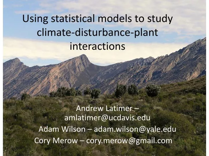
Using statistical models to study climate-disturbance-plant interactions. Andrew Latimer – amlatimer@ucdavis.edu Adam Wilson – adam.wilson@yale.edu Cory Merow – cory.merow @gmail.com. Mediterranean climate. Key features: warm temperate, with cool wet winters and hot dry summers.

E N D
Using statistical models to study climate-disturbance-plant interactions Andrew Latimer – amlatimer@ucdavis.edu Adam Wilson – adam.wilson@yale.edu Cory Merow – cory.merow@gmail.com
Mediterranean climate • Key features: warm temperate, with cool wet winters and hot dry summers.
Climate change effects? The obvious ones: • Warmer winter -> more growth • Hotter summer -> more fire
Complications May raise growth rate while hammering other parts of life cycle (e.g. survival) Fire-plant feedbacks can produce rapid shift -> fuel starvation -> flammability
Feedback example – Sierra forest • When feedbacks positive, slight shift in disturbance regime can cause state change Moderate fire e.g. Collins et al. (2009) Ecosystems (-) Less fuel, milder fire Intense fire e.g. Stevens et al. (2013) Can.J.For.Res. (+) More shrubs, intense fire Photos: Jens Stevens
Fire-plant interaction example: South African fynbos No fire (fire suppressed) No fire (plant growth suppressed) Fire
More frequent fire can eliminate populations 8-year intervals 4-year intervals between fires between fires Population size Stevens & Beckage, Oecologia 2010
Climate Growth, Survival etc. Ignition and spread Plant species, communities Fire Disturbance Regrowth of Fuel, flammability
Challenges – ecological data • Scales of process can be large • Field data collection is almost always not • Interpolation and extrapolation (worse in projections) Current Future Environment
Challenges – environmental data • Highly multivariate environmental measurements • Sensor outputs • Model outputs • Heterogeneous data sources • Multivariate responses • Community: Many species, life stages • Individual: phenotypes, genotypes • What’s important and why? • Q: Are the factors on both sides sparse?
Outline • A little more introduction • Fire return times • Biomass regrowth • Demography
Study system for this talkCape Floristic Region of South Africa • Fynbosshrubland interfacing with karroodesert • Evolutionary radiation-> very high plant diversity and endemism • Diversity concentrated in ~30 lineages over 0.5-30 MY
CFR climate change Historical patterns Recent change (1950-2000) Change per decade (mm)
Climate change projectionsCMIP5 multimodel average 2081-2100 -- RCP8.5 Stippling: ≥ 8/11 models agree on sign Downscaled projections: Adam Wilson
Thomas et al. (2004) Nature.Midgleyet al. (2006). Diversity & Distributions.
Example 1: Fire occurrenceWhat affects fire frequency? Climate Growth, Survival etc. Ignition and spread Plant species, communities Fire Disturbance Regrowth of fuel
Cape region fire data Thanks to Helen DeKlerk
Fire data preparation • Overlay ~2km x 2km grid on reserve areas • Seasonal time resolution (3 months) • Cell considered “burned” if >50% area burned • Voxels of weather data: • 80 seasons x 2611 cells = 208,880 voxels
Issues… • Very multivariate weather data • Approach: reduce dimensionality by biological intuition, hypothesis • Chris Wikle:“Sensible science-based parameterizations or dimension reductions”
Issue: highly multivariate environmental data Bayesian kriging with covariates (Adam Wilson) Weather station data Daily, point locations Gridded weather data Daily, ~2km grid Meetings (many…) Soil moisture model Choice of methods Modeling Indices -- i.e. hypotheses Seasonal to yearly
Fire history data Timeline for one grid cell 6 years 14 years ? ? 2000 (end of record) 1980 (beginning of record) fires Other hypothetical fire histories: .
Nonparametric survival model Zi = observed time between a pair of fires in cell I Pit : P(Zi > t | Zi > t-1) i.e. probability of “surviving” season t without a fire Probit(P) = XTβ + e Climate: Long-term mean Weather: anomalies in each grid cell * season Climate index (AAO) Random effects: season, sub-region Note Alan Gelfand’s 2013 paper adding spatial random effects
Dealing with censoring • Left censoring: no previous fire observed in record Unobserved pit predicted from XTβ {Unobservedfire times} ~ Multinom(1-pit, t in [1950-1979]) Gives length distribution of unobserved fire intervals # Note may inflate fire frequency because a few cells will have failed to burn in these 30 years
? Wilson et al. (2010) Ecological Modelling
Cumulative fire probabilities Wilson et al. (2010) Ecological Modelling
Expected fire return times Wilson et al. (2010) Ecological Modelling
Importance of large-scale atmospheric circulation patterns • Importance of AAO brings us back to complex multivariate problem (why AAO??) • But in this case pretty clear how it works
Note trends in ozone depletion (ozone hole) associated with positive AAO • Manatsaet al. (2013) Nature Geosci. Abram, et al. (2014) Nature Climate Change doi:10.1038/nclimate2235
Part 2: modeling postfire regrowth Climate Growth, Survival etc. Ignition and spread Plant species, communities Fire Disturbance Regrowth of fuel
Remote sensing: Watching plants grow from space • MODIS terra NDVI data
Model • Functional form that can match recovery pattern • Parameters • αi : minimum NDVI • γi: difference between min and max NDVI • λi: recovery rate parameter • Αi: amplitude of seasonal variation
Wet, coastal ~4 years Dry, interior ~8 years Wilson et al. in prep
Spatial variation in regrowth rates Regrowth rate based on Threshold NDVI value (95% of max NDVI) Wilson et al. in prep
Tying this back to demographic modelsFactors related to regrowth rate Wilson et al. in prep
Projected change in recovery time longer Years shorter
Comparing recovery time to observed fire return intervals Some correspondence Slowest growing areas may be burning too often
Conclusions on fire • Climate change likely to shorten fire return times • And also increase regrowth rates in many areas • But: Lower warm-season precipitation in the west, hotter summers • Big shifts possible • Frequent fire in slow-recovery areas • Fuel starvation and fynboscontraction (?)
Example 3: Demography Tradeoff: -- More biological detail -- MUCH less data Climate Growth, Survival etc. Ignition and spread Plant species, communities Fire Disturbance Regrowth of fuel
Focal species: Protearepens Data: Protea Atlas Project Tony Rebelo of SANBI
Goal: model population performance across region • Measure across gradients • Demographic rates: • Growth & Fecundity • Mortality (dead adults) • Recruitment (seedlings per parent) Issue: recruitment sites limited by fire occurrence
Analysis issues • Misalignment • Growth and seed production measured at different sites from seedling recruitment • Missing some steps in life cycle • Seedling emergence and survival Scaling issues raised by Jim and Alan
Integral projection model (IPM) t = time z = size at t z' = size at t+1 nt(z) = size distribution of individuals at t nt+1(z’) = size distribution of individuals at t+1 K(z’,z) = projection kernel
Life History: Perennial shrub state vector “kernel” P(z’,z) = (survival) * (growth) F(z’,z) = (mean # flowers/plant) * (mean # seeds/flower) (establishment probability)* (offspring size)
Jump into the bog of elasticity Merowet al. 2014 Ecography
Mean modeled pop growth rate If we treat this as species distribution model And assume presence predicted where λ ≥ 1.0 Merowet al. 2014 Ecography