Download
1 / 26
270 likes | 386 Views
Imaging from Projections. Eric Miller With minor modifications by Dana Brooks. Outline. Problem formulation What’s a projection? Application examples Why is this interesting? The forward problem The Radon transform The Fourier Slice Theorem The Inverse Problem

E N D
Imaging from Projections Eric Miller With minor modifications by Dana Brooks These slides based almost entirely on a set provided by Prof. Eric Miller
Outline • Problem formulation • What’s a projection? • Application examples • Why is this interesting? • The forward problem • The Radon transform • The Fourier Slice Theorem • The Inverse Problem • Undoing the Radon transform with the help of Fourier • Filtered Backprojection Algorithm • Complications and Extensions These slides based almost entirely on a set provided by Prof. Eric Miller
t y x A Projection The total amount of f(x,y) along the line defined by t and q These slides based almost entirely on a set provided by Prof. Eric Miller
Application Examples • CAT scans: • X ray source moves around the body • f(x,y) is the density of the tissue • MRI • Not as clear cut what the “projection” is, but in a peculiar way, the math is the same (remind me to talk about this when we get to the MRI Imaging equation …) • f(x,y) is the spin density of molecules in the tissue • Synthetic Aperture Radar • Satellite moves down a linear track collecting radar echoes of the ground • Used for remote sensing, surveillance, … • Again: math is the same (after much pain and anguish) • f(x,y) is the reflectivity of the earth surface These slides based almost entirely on a set provided by Prof. Eric Miller
Motivation • In all cases, one observes a bunch of sum or integrals of a quantity over a region of space: these are “projections” • The goal is to use a collection of these projections to recover f(x,y). • Here we will talk about the full data case • Assume we see for all q and t • Limited view tomography a topic for advanced course These slides based almost entirely on a set provided by Prof. Eric Miller
t y x The Radon Transform Polar equation for line: So the line exists only where this equation is true Function oft and q These slides based almost entirely on a set provided by Prof. Eric Miller
What does it do? Simplest case: f(x,y) a d function: only exists at a single point • Proof only by limiting argument as products of d’s not well defined • Interpretation: • A “function” in (t,q) space which “is” 1 along a sinusoidal curve and zero elsewhere: note that a point in 2D a curve • Say y0 = 0 and x0 = 1 then this is an “image” which “is” 1 whent = cos q These slides based almost entirely on a set provided by Prof. Eric Miller
Note that we draw as a rectangular “image” in t and q In Pictures Kind of 2D impulse response (PSF) y t q x The Image Called the Radon Transform (a.k.a.the sinogram) These slides based almost entirely on a set provided by Prof. Eric Miller
More Examples t q t q These slides based almost entirely on a set provided by Prof. Eric Miller
Fourier Slice Theorem • Key idea here and for a large number of other problems • Analytically relate the 1D Fourier transform of P to the 2D Fourier transform of f. • Why? • If we can do this, then a simple inverse 2D Fourier gives us back f from the “data” P. These slides based almost entirely on a set provided by Prof. Eric Miller
Recall 2D Fourier Transform Analysis Synthesis • “Space” variable x goes with “frequency” variable u • “Space” variable y goes with “frequency” variable v • (u,v) called “spatial frequency domain” These slides based almost entirely on a set provided by Prof. Eric Miller
Fourier – Slice Theorem (FST) • Let F(u,v) be defined as on last slide • Define Sq(w) as the 1D Fourier transform of P along t • for some frequency variable w • FST says that Sq is equal to F(u,v) along a line • tilted at an angle q with respect to the (u,v) • coordinate system • To make this more precise … These slides based almost entirely on a set provided by Prof. Eric Miller
v F(u,v) along line w u Fourier-Slice t 1D Fourier Transform y x Variables w and q are the polar form of u and v So FST is: These slides based almost entirely on a set provided by Prof. Eric Miller
Reconstruction Implications v • Collect data from lots and lots of projections. • Take 1D FT of each to get one line in 2D frequency space • Fill up 2D spatial frequency space on a polar grid • Interpolate onto rectangular grid • Inverse 2D FT and we are done!! u These slides based almost entirely on a set provided by Prof. Eric Miller
An Alternate ApproachFiltered Backprojection • This requires lots of Fourier Transforms • This means we can’t begin processing until we have all slices • Turns out there’s a more efficient way to organize things • This requires “ugly” interpolation, worse at high frequencies The derivation of this algorithm is perhaps one of the most illustrative examples of how we can obtain a radically differentcomputer implementation by simply re-writing the fundamentalexpressions for the underlying theory - Kak and Slaley, CTI These slides based almost entirely on a set provided by Prof. Eric Miller
w FBP Motivation in Pictures v v w u u • In practice, we measure over lines. • Idea: build a 2D filter which covers the line, but has the same “weight” as the wedge at that frequency, w • In other words “mush” triangle to a rectangle • Then “sum up” filtered projections By linearity, could in theory break up reconstruction intocontribution from independent“wedges” in 2D Fourier space • For K projections, the width of the wedge at w is just These slides based almost entirely on a set provided by Prof. Eric Miller
FBP Theory Now, change right side from polar to rectangular To get rectangular coordinates in space, polar in frequency: These slides based almost entirely on a set provided by Prof. Eric Miller
FBP Theory II Make use of two facts: To arrive at Backproject Filter (in space) These slides based almost entirely on a set provided by Prof. Eric Miller
w FBP Interpretation • Recall from linear systems • So |w| filter is more or less a differentiator. Accentuated high frequency information leads to problems with noise amplification • In practice, roll off response. w These slides based almost entirely on a set provided by Prof. Eric Miller
FBP Interpretation Backprojection: Note that Qq(t) needs only one (filtered) projection Think of this as Qq(t) evaluated at the point t = xcosq + y sinq Sum up over allangles t • Along this line in “image space” set the value to • Qq(t0) • All points get a value • Do for all angles • Add up y Region we arereconstructing x These slides based almost entirely on a set provided by Prof. Eric Miller
FBP Example Orig. Recon Zoom These slides based almost entirely on a set provided by Prof. Eric Miller
Limited data I:Angle decimation These slides based almost entirely on a set provided by Prof. Eric Miller
Limited data II:Limited Angle These slides based almost entirely on a set provided by Prof. Eric Miller
Artifact Mitigation • Take a more matrix-based “inverse problems” perspective • Discretized Radon transform, data, and object to arrive at a forward model • Where C has many fewer rows than columns • Use SVD, TSVD, Tikhonov, or other favorite regularization scheme to improve reconstruction results • Note: significant move from analytical to numerical inversion means a basic shift in how we are approaching the problem. No more FBP (at least not easily) These slides based almost entirely on a set provided by Prof. Eric Miller
Other Fourier Imaging Applications v v u u • Diffraction tomography • Collects data on petal shaped regions of Fourier space • Very limited view • More sophisticated math than X ray • Arises in geophysical and medical imaging problems • Standard SAR • Collects data on wedge shaped regions of Fourier space • Very limited view • Similar math to X-ray These slides based almost entirely on a set provided by Prof. Eric Miller
Generalized Radon Transforms • Radon transform = integral of object over straight lines • Many extensions • Integration over planes in 3D • Over circles in 2D (different type of SAR) • Over much more arbitrary mathematical structures (asymptotic case of some acoustics problems with space varying background). • Of weighted object function (attenuated Radon transform) These slides based almost entirely on a set provided by Prof. Eric Miller