Download
1 / 39
420 likes | 753 Views
Quandles & Q -colouring of knots. Krzysztof Putyra Jagiellonian University 21 st September 2006. f. An embedding f : 1 3 is a knot if it is smooth or PL. X = { f : 1 3 | f is a knot } – a knot space. Knots & diagrams.

E N D
Quandles&Q-colouring of knots Krzysztof Putyra Jagiellonian University 21st September 2006
f An embedding f : 13 is a knot if it is smooth or PL. X = {f : 13|f is a knot} – a knot space Knots & diagrams Two knots are equivalent iff lies in the same path component of X.
p tunnels bridge Knots & diagrams This gives us a diagram of a knot.
Knots & diagrams unknot trefoil figure-eight knot cinquefoil
Knots & diagrams Theorem (K. Reidemeister, 1927). Let K1, K2 be knots with diagrams D1, D2. Then K1, K2 are equivalent iff D1 can be obtained from D2 by a finite sequence of moves, called Reidemeister moves: Kurt Reidemeister R1 R2R3
f Fox’sn-colourability crossing relations
Fox’sn-colourability What are the crossing relations? A n-colouring is trivial if it uses only one colour. A knot is n-colourable if its diagram posses any non-trivial n-colouring.
crossing relation: Understand colourings How to compute n-colourings? 0 b 1 4 a c = ? 2 3
0 1 4 2 3 Rows are lin.dep. delete first row Set c1 = 0 delete first column Understand colourings c4 c1 c2 c3 c5 detK := |detA+| is invariant under Redemeister moves. It is called the determinant of a knot.
Understand colourings Theorem. Knot K is n-colourable iff GCD(detK, n) ≠ 1. Proof. We need to solve in n the equation: A+c = 0 There exist matrices B, C, D such that D = BA+CD = diag(d1,…,dl) where B, C are isomophisms and detD = detA+. Now kerA+ kerD and kerD ≠ 0 i: GCD(di, n) ≠ 1 GCD(detK, n) ≠ 1 31 & 51
Understand colourings det = det = 5 Colourings cannot distinguish these knots! What can be changed to improve colourings? Crossing relations!
cov cr cl Improving colourings Having the set of colours C, define the crossing relation in the following way: clcov = cr for some operation : C×C C. Which properties such an operation must have, to produce some natural invariants?
cov cr cl Improving colourings Conditions for: C×C C: clcov = cr
cov cr cl Improving colourings • Conditions for: C×C C: • Q1: x x = x clcov = cr x x x x x
cov cr cl Improving colourings • Conditions for : C×C C: • Q1: x x = x • Q2: unique z: z x = y clcov = cr x y x y where ax = y x x y x a
cov cr cl Improving colourings • Conditions for : C×C C: • Q1: x x = x • Q2: unique z: z x = y • Q3:(z y) x = (z x) (y x) clcov = cr x x y y where z’ = (z x) (yx) z” = (z y) x z z z’ z” x x y x y x
cov cr cl Improving colourings • Conditions for : C×C C: • Q1: x x = x • Q2: unique z: z x = y • Q3:(z y) x = (z x) (y x) • To make computings easy, we like: • Q4: : C×C C is linear clcov = cr
Quandles – definitions • A quandle is a set Q equipted with a binary operation • : Q×Q Qsuch that for all a,b,c Q: • Q1: a a = a (idempotent) • Q2: exists uniquex: x a = b (left-invertible) • Q3: (a b) c = (a c) (b c) (self-distributive) • A quandle (Q,)is called linear if Q is a ring and • Q4: : Q×Q Q is linear Define :Q×QQas follow: (ab) b = a The pair (Q, ) is called a dual quandle to (Q, ).
what gives under Q2: In a similar way one can check, that is additive. Quandles – properties Theorem. A quandle dual to a linear quandle is linear. Proof. Let (Q, ) be a linear quandle with dual (Q, ). Then for a, x, y Qwe have:
Proof. Let (Q, ) be a linear quandle with dual (Q, ). Then for x, y Q we have: what gives under Q2: This shows that operation is dual to . Quandles – properties Theorem. An operation of duality is an involution.
Quandles – examples background structurexy xy discrete quandle X – any set x x conjugative quandle G – a groupy-1xy yxy-1 dihedral quandle n – a ring 2y – x 2y – x R – a ring, s – unit (1–s)y + sx (1–s-1)y + s-1x Alexander quandle = [t±1] (1–t)y + tx (1–t-1)y + t-1x
Q-colourability Q-colouring – a function from arcs of a diagram into a quandle Q. b = ? crossing relations: ca = b ba = c a c = ? A Q-colouring is trivial if it uses only one colour. A diagram is Q-colourable if it posses any non-trivial Q-colouring.
Rows are lin.dep. delete first row Set c1 = 0 delete first column Q-colourability c4 colouring with (22, ) xy = 7x – 6y c1 c2 c3 c5 detQK := detA+ is invariant under Redemeister moves (with accurancy to units). It is the Q-determinant of a knot.
Module of Q-colurings: colQD = kerA Q-module of a diagram: Qn = (x1,…, xn : r1 = … = rm = 0) modQD = imA Q-colourability D – a diagram with n arcs and m crossings Q– a linear quandle A– a matrix generated by crossing relations
Q-colourability Theorem. For a diagram D and a linear quandle Q: colQD Hom(modQD; Q) Proof: Let modQD = (m1,…,mn : r1 = … = rm = 0). For f: modQD Qdefine a Q-colouring f̃ as f̃ (xi) := f (mi). Also every Q-colouring f̃ induces a homomorphism s.th. f (mi) := f̃(xi) That is because for any relation ri = x y – z we have f (ri) = f (x) f (y) – f (z) = f̃(x) f̃ (y) – f̃(z) = 0.
Q-colourability Theorem. The Q-module of a diagram is invariant under Reidemeister moves. Colloary. The module of Q-colourings of a diagram is a knot invariant. Proof.Let D1 and D2 be diagrams of a knot K. Then colQD1 Hom(modQD1; Q) Hom(modQD2; Q) colQD2
14 2 0 10 Q-colourability Consider quandle22 with an operation: Cinquefoil does not posses non-trivial 22-colouring, in opposition to the figure-eight knot.
Q-colourability Knots colourable with no linear quandles exist!
Q-colourability • Further improvements: • modules with a Q-structure • non-commutative rings • relations of another type
References • R. H. Crowell, R. H. Fox, An introduction to knot theoryGinn. and Co., 1963 • L. Kauffman, On knotsAnnals of Math. Studies, 115, Princeton University Press, 1987 • L. Kauffman, Virtual knots theoryEurop. J. Combinatorics (1990) 20, 663-691 • B. Sanderson, Knots theory lectures http://www.maths.warwick.ac.uk/~bjs/ • S. Nelson, Quandle theoryhttp://math.ucr.edu/~snelson/
Thank you for your attention