Download
1 / 36
360 likes | 479 Views
Correlation. ... beware. Definition. Var (X+Y) = Var (X) + Var (Y) + 2·Cov(X,Y) The correlation between two random variables is a dimensionless number between 1 and -1. Interpretation. Correlation measures the strength of the linear relationship between two variables. Strength

E N D
Correlation ... beware
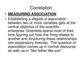
Definition Var(X+Y) = Var(X) + Var(Y) + 2·Cov(X,Y) The correlation between two random variables is a dimensionless number between 1 and -1.
Interpretation Correlation measures the strength of the linear relationship between two variables. • Strength • not the slope • Linear • misses nonlinearities completely • Two • shows only “shadows” of multidimensional relationships
A correlation of +1 would arise only if all of the points lined up perfectly. Stretching the diagram horizontally or vertically would change the perceived slope, but not the correlation.
A positive correlation signals that large values of one variable are typically associated with large values of the other. Correlation measures the “tightness” of the clustering about a single line.
A negative correlation signals that large values of one variable are typically associated with small values of the other.
But a correlation of 0 most certainly does not imply independence. Indeed, correlations can completely miss nonlinear relationships.
Correlations Show (only)Two-Dimensional Shadows In the motorpool case, the correlations between Age and Cost, and between Make and Cost, show precisely what the manager’s two-dimensional tables showed: There’s little linkage directly between Age and Cost. Fords had higher average costs than did Hondas. But each of these facts is due to the confounding effect of Mileage! The pure effect of each variable on its own is only revealed in the most-complete model.
Potential for Misuse (received via email from a former student, all employer references removed) “One of the pieces of the research is to identify key attributes that drive customers to choose a vendor for buying office products. “The market research guy that we have hired (he is an MBA/PhD from Wharton) says the following: “‘I can determine the relative importance of various attributes that drive overall satisfaction by running a correlation of each one of them against overall satisfaction score and then ranking them based on the (correlation) coefficient scores.’ “I am not really certain if we can do that. I would tend to think we should run a regression to get relative weightage.”
Customer Satisfaction • Consider overall customer satisfaction (on a 100-point scale) with a Web-based provider of customized software as the order leadtime (in days), product acquisition cost, and availability of online order-tracking (0 = not available, 1 = available) vary. • Here are the correlations: • Customers forced to wait are unhappy. • Those without access to online order tracking are more satisfied. • Those who pay more are somewhat happier. • ?????
The Full Regression Customers dislike high cost, and like online order tracking. Why does customer satisfaction vary? Primarily because leadtimes vary; secondarily, because cost varies.
Reconciliation • Customers can pay extra for expedited service (shorter leadtime at moderate extra cost), or for express service (shortest leadtimeat highest cost) • Those who chose to save money and wait longer ended up (slightly) regretting their choice. • Most customers who chose rapid service weren’t given access to order tracking. • They didn’t need it, and were still happy with their fast deliveries.
Finally … • The correlations between the explanatory variables can help flesh out the “story.” • In a “simple” (i.e., one explanatory variable) regression: • The (meaningless) beta-weight is the correlation between the two variables. • The square of the correlation is the unadjusted coefficient of determination (r-squared). • If you give me a correlation, I’ll interpret it by squaring it and looking at it as a coefficient of determination.
A Pharmaceutical Ad Diagnostic scores from sample of patients receiving psychiatric care So, if your patients have anxiety problems, consider prescribing our antidepressant!
Evaluation • At most 49% of the variability in patients’ anxiety levels can potentially be explained by variability in depression levels. • “potentially” = might actually be explained by something else which covaries with both. • The regression provides no evidence that changing a patient’s depression level will cause a change in their anxiety level.
Association vs. Causality • Polio and Ice Cream • Regression (and correlation) deal only with association • Example: Greater values for annual mileage are typically associated with higher annual maintenance costs. • No matter how “good” the regression statistics look, they will not make the case that greater mileage causes greater costs. • If you believe that driving more during the year causes higher costs, then it’s fine to use regression to estimate the size of the causal effect. • Evidence supporting causality comes only from controlled experimentation. • This is why macroeconomists continue to argue about which aspects of public policy are the key drivers of economic growth. • It’s also why the cigarette companies won all the lawsuits filed against them for several decades.
Modeling: Variable Selection Request: “Estimate the annual maintenance costs attributable to annual mileage on a car. Dollars per thousand miles driven will suffice.” This sounds like a regression problem! Let’s sample some cars, and look at their costs and mileage over the past year.
The Results This all looks fine. And it’s wrong!
Here’s What the Computer Sees: What it doesn’t see is the age bias in the data: The cars to the left are mostly older cars, and the cars to the right are mostly newer. An un(age)biased chart would have some lower points on the left, and some higher points on the right … and the regression line would be steeper.
Specification Bias • … arises when you leave out of your model a potential explanatory variable that (1) has its own effect on the dependent variable, and (2) covaries systematically with an included explanatory variable. • The included variable plays a double role, and its coefficient is a biased estimate of its pure effect. • That’s why, when we seek to estimate the pure effect of one explanatory variable on the dependent variable, we should use the most-complete model possible.
Seeing the Man Who isn’t There Yesterday, upon the stair, I met a man who wasn’t there He wasn’t there again today I wish, I wish he’d go away... Antigonish (1899), Hughes Mearns When doing a regression study in order to estimate the pure effect of some variable on the dependent variable, the first challenge in the real (non-classroom) world is to decide for what variables to collect data. The “man who isn’t there” can do you harm. Let’s return to the motorpool example, with Mileage as the only explanatory variable, and look at the residuals, i.e., the errors our current model makes in predicting for individuals in the sample.
Learning from our Mistakes Take the “residuals” output Sort the observations from largest to smallest residual. And see if something differentiates the observations near the top of the list from those near the bottom. If so, consider adding that differentiating variable to your model!
We Can Do This Repeatedly Our new model: After sorting on the new residuals, 3 of the top 4 and 5 of the top 7 cars (those with the greatest positive residuals) are Hondas. 3 of the bottom 4 and 5 of the bottom 7 cars (those with the greatest negative residuals) are Fords. This might suggest adding “make” as another new variable.
Why Not Just Include the Kitchen Sink? • Spurious correlation • The Dow, and women’s skirts • Colinearity • For example, age and odometer miles: Likely highly correlated • Computer can’t decide what to attribute to each • Large standard errors of coefficients leads to large significance levels = no evidence either belongs. • But if either is included alone, strong evidence it belongs
Structural Variations • Interactions • When the effect of one explanatory variable on the dependent variable depends on the value of another explanatory variable • The “trick”: Introduce the product of the two as a new artificial explanatory variable. Example • Nonlinearities • When the impact of an explanatory variable on the dependent variable “bends” • The “trick”: Introduce the square of that variable as a new artificial explanatory variable. Example
Interactions: Summary • When the effect (i.e., the coefficient) of one explanatory variable on the dependent variable depends on the value of another explanatory variable • Signaled only by judgment • The “trick”: Introduce the product of the two as a new artificial explanatory variable. After the regression, interpret in the original “conceptual” model. • For example, Cost = a + (b1+b2Age)Mileage + … (rest of model) • The latter explanatory variable (in the example, Age) might or might not remain in the model • Cost: We lose a meaningful interpretation of the beta-weights
Examples from the Sample Exams Caligula’s Castle: Revenuepred = -1224.82 + 62.37Age – 0.5201Age2– 121.9Sex + 1.99Direct + (0.8527+1.4377Sex)Indirect Give direct incentives (house chips, etc.) to men Give indirect incentives (flowers, meals) to women The Age effect on Revenue is greatest at Age = -(62.37)/(2(-0.5201)) = 59.96 years
Examples from the Sample Exams Hans and Franz: CustSatpred = 84.40 – 0.8667Wait – 0.0556Wait2 – 5.602Size + (-40.0845+8.7747Size)Franz? Set Franz? = 0 (assign Hans) when the party size is < 40.0845/8.7747 = 4.568 Customers’ anger grows more quickly the longer they wait
Nonlinearity: Summary • When the direct relationship between an explanatory variable and the dependent variable “bends” • Signaled by a “U” in a plot of the residuals against an explanatory variable • The “trick”: Introduce the square of that variable as a new artificial explanatory variable: Y = a + bX + cX2 + … (rest of model) • One trick can capture 6 different nonlinear “shapes” • Always keep the original variable (the linear term, with coefficient “b”, allows the parabola to take any horizontal position) • c (positive = upward-bending parabola, negative = downward-bending) • -b/(2c) indicates where the vertex (either maximum or minimum) of the parabola occurs • Cost: We lose a meaningful interpretation of the beta-weights
Examples from the Sample Exams Caligula’s Castle: Revenuepred = -1224.82 + 62.37Age – 0.5201Age2– 121.9Sex + 1.99Direct + (0.8527+1.4377Sex)Indirect Give direct incentives (house chips, etc.) to men Give indirect incentives (flowers, meals) to women The Age effect on Revenue is greatest at Age = -(62.37)/(2(-0.5201)) = 59.96 years
Examples from the Sample Exams Hans and Franz: CustSatpred = 84.40 – 0.8667Wait – 0.0556Wait2 – 5.602Size + (-40.0845+8.7747Size)Franz? Set Franz? = 0 (assign Hans) when the party size is < 40.0845/8.7747 = 4.568 Customers’ anger grows more quickly the longer they wait
Sample Datasets • Four datasets continuing to review material from Session 2, with some added modeling issues. • Two very thorough sample exams. • One based on Harrah’s success in understanding its patrons • One based on a restaurateur comparing maitresd’hotel, with a 90-minute prerecorded Webex tutorial