Download
1 / 37
380 likes | 502 Views
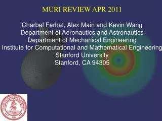
MURI REVIEW APR 2011 Charbel Farhat , Alex Main and Kevin Wang Department of Aeronautics and Astronautics Department of Mechanical Engineering Institute for Computational and Mathematical Engineering Stanford University Stanford, CA 94305. OUTLINE. Review of FVM-ERS method.

E N D
MURI REVIEW APR 2011 CharbelFarhat, Alex Main and Kevin Wang Department of Aeronautics and Astronautics Department of Mechanical Engineering Institute for Computational and Mathematical Engineering Stanford University Stanford, CA 94305
OUTLINE • Review of FVM-ERS method • Implementation of exact Riemann solver (ERS) for Tait • -JWL interfaces • Implementation of programmed burn method in AERO-F • Theory • Numerical Examples • Implementation of one dimensional simulations
1 1 Fj,j+1 = Fj+1/2 (nj,j+1) = (Fj+ Fj+1 )- | F’ |j+1/2 (Wj+1 – Wj) = Roe (Wj, Wj+1, gs, ps) (stiffenedgas) 2 2 @(rf) (ruf) @ + = 0 @t @x COMPUTATIONAL FRAMEWORK • MUSCL-based solver with Roe Flux j + 1/2 j j + 1 • Interface capturing via the level-set equation (conservation form)
FVM-ERS • FVM with exact local Riemann solver for multi-phase flows Wjn W*n W*n Wj+1n j - 1 j - 1/2 j j + 1/2 j + 1 - Fj,j+1 = Roe (Wjn, W*n, EOSj) Fj+1,j = Roe (Wj+1n, W*n, EOSj+1) - W*n and W*n determined from the exact solution of local two-phase Riemann problems C. Farhat, A. Rallu and S. Shankaran, "A Higher-Order Generalized Ghost Fluid Method for the Poor for the Three-Dimensional Two-Phase Flow Computation of Underwater Implosions", Journal of Computational Physics, Vol. 227, pp. 7674-7700 (2008)
Wnpj+1 Wnpj • Exact solution of the analytical problem (Tait’s EOS) 1 1 (RR(pI; pR,rR) - RL(pI; pL,rL)) uI = (uL + uR) + 2 2 RL(pI; pL,rL) + RR(pI; pR,rR) + uR – uL = 0 pI, rIL, rIR, uI - Newton’s method EXACT RIEMANN SOLVER • Wave structure and Riemann problem rIL,pI,uI ,rIR contact discontinuity rarefaction shock t gas water x j j + 1/2 j + 1 rLuL pL rRuR pR
EQUATIONS OF STATE • Stiffened Gas p = re(g - 1)+gp • Also support Tait EOS for compressible liquids p = Arb + B • Jones-Wilkins-Lee equation of state for explosive • products • Perfect Gas (PG) is a subset of SG (with p = 0)
p = A(1 - )e-R1+ B(1 - )e-R2 + wre wr wr R1r0 R2r0 r0 r0 r r JWL EOS • Jones-Wilkins-Lee (JWL) equation of state for modeling explosive products of combustion (and in particular Trinitrotoluene — a.k.a. TNT) where A, B, R1, R2, w and r0 are material constants - Highlynonlinearfunctionp(r,e) - Presence of exponentials
uL + FL(rL, pL;rIL) = uIL = uIR = uR + FR(rR, pR; rIR) GL(rL, pL; rIL) = pIL pIR= GR(rR, pR; rIR) = TAIT-JWL ERS • FVM-ERS needs an exact Riemann solver for problems • involving interfaces between fluids modeled as Tait and • fluids modeled as JWL • Solution of exact Riemann problem involves a • system of two nonlinear equations (1) (2) • FL and GL depend on the nature of the interaction in the • phase modeled by the JWL EOS • shock algebraic equation • rarefaction differential equation
rIR,uIR ,pIR t rarefaction c(r,p) rR,uR ,pR = r x du + _ dr = s rw+1 p - Ae-R1+ Be-R2 r0 r0 r r TAIT-JWL RIEMANN SOLVER • Rarefaction wave in a JWL medium (k) • The isentropic evolution in the • rarefaction fan between two • constant states is given by (1) (2) complex Riemann problem • Algebraic entropy (s) formula for the JWL EOS • No obvious algebraic Riemann invariants for the JWL EOS • No analytical Jacobians of the invariants either
JWL EOS • Riemann invariants are tabulated for the explicit • time stepping scheme • For implicit time-stepping, where Jacobians are • required, they are not tabulated; rather they are • computed on-line by solving an ODE • Relatively cheap compared to other aspects of • the simulation • Support both SG-JWL and JWL-JWL
SHOCK TUBE PROBLEM • 1D Shock tube with TNT gaseous products to the left at • high pressure, and water at low pressure to the right • Water modeled using Tait equation of state • ( r0 = 1000 kg/m3, p0 = 100 kPa, B = 331 MPa ) • TNT gaseous products modeled using JWL equation • of state • A = 548.4 GPa • B = 9.375 Gpa • R1 = 4.94 • R2 = 1.21 • w = 0.28 • r0 = 1630 kg/m3
r = 1630 (kg/m3) r = 1000.0 (kg/m3) u= 0.0 (m/s) u= 0.0 (m/s) p= 7.81 x 10⁹ (Pa) p= 105(Pa) SHOCK TUBE PROBLEM • pL = 7.81 GPa, rL= 1630 kg/m3, uL= 0 pR = 1 kPa, rR= 1000 kg/m3, uR= 0 TNT products Water • Simulation to t = 5 x 10⁻⁴s in 3D AERO-F code
PROGRAMMED BURN • Simulate detonation of high explosives • Motivated because detonation products generally have • varying fluid state
CHAPMAN-JOUGUET THEORY • The simplest model of detonation waves is due to • Chapman-Jouguet (CJ) theory. Unburned HE r0, p0, u0=0 Burned Products rCJ, pCJ, uCJ s - Detonationwave has constant velocity (s) - Assumes thatgaseousproductsjustbehind the detonationwave move atsonicvelocity - Implies s = uCJ + cCJ
CHAPMAN-JOUGUET THEORY • Post-detonation state ( rCJ, pCJ, uCJ) then comes from • the Rankine-Hugoniot relations: rCJ (uCJ– s) = - r0 s pCJ+ rCJ(uCJ– s)2 = p0+ r0s2 eCJ+ + (uCJ– s)2= e0 + + s2 pCJ p0 1 1 rCJ r0 2 2 • Where e0 is the detonation energy associated with the • unburned high explosive
PROGRAMMED BURN • Numerical method • Similar to “Change in EOS” method in GEMINI • Extended to handle more general cases • General idea – prescribe constant speed of detonation • front • When the detonation front passes a cell, change the • equation of state for that cell from unburned to burned
PROGRAMMED BURN • Fluxes are computed with FVM-ERS • What about interface tracking? • Possible for 3 phases to meet at a single point
INTERFACE TRACKING • We only track interface between explosive (burned AND • unburned) and water • Already know where interface between burned and • unburned explosive is!
PHASE CHANGE • Phase change occurs when the level set at a node • changes sign - Nodeinsidedetonationwave -> burned explosive - Nodeoutsidedetonationwave-> unburned explosive • Also occurs when detonation wave passes a node • containing unburned explosive - Conservative variables are not changed - In contrast to usual FVM-ERS method
EXPLOSIVE MODELING • Burned products can be modeled with either JWLor • ideal gas equations of state • Unburned explosive modeled with Tait equation of state p = Arb + B - A, B chosensothat (r0, p0) and (rCJ, pCJ) are admissible states - Internalenergy set to be e0 (detonationenergy)
NUMERICAL EXAMPLES • One dimensional TNT planar burn • Three dimensional TNT spherical burn • Detonation of TNT cube • Asymmetrical (TNT) charge near flexible structure
1D PLANAR BURN • One dimensional TNT planar burn,surrounded by water • TNT gaseous products modeled using JWL equation of • state, water by stiffened gas (g = 4.4, p = 6.0 x 10⁸) Explosive Water Water Explosive r0 = 1630 kg/m3 p0 = 100 kPa e0 = 3.68 MJ Water r0 = 1000 kg/m3 p0 = 100 kPa
TNT MODEL • TNT modeled by JWL equation of state: • A = 548.4 GPa • B = 9.375 Gpa • R1 = 4.94 • R2 = 1.21 • w = 0.28 • r0 = 1630 kg/m3 • Chapman-Jouguet Theory says that • s = 6930 m/s • - pCJ = 20.9 GPa • - rCJ = 2100 kg/m3
SPHERICAL BURN • Simulation of a spherical (slice) charge in 3D 0.15 m 0.25 m Explosive r0 = 1630 kg/m3 p0 = 100 kPa e0 = 3.68 MJ Water r0 = 1000 kg/m3 p0 = 100 kPa
SPHERICAL BURN • AERO-F burn results nearly identical to those obtained • by GEMINI • Burn pressure peak is slightly lower; AERO-F mesh is • slightly coarser • AERO-F mesh size – Dr = 0.5 cm • GEMINI mesh size – Dr = 0.25 cm • Discrepancy in the shock propagation in the water • AERO-F uses stiffened gas EOS • GEMINI uses Tillotson EOS
ASYMETRICAL BURN • Detonation of a cube of TNT, surrounded by water Solid Symmetry Water Solid Symmetry Explosive • Domain is 1 m / side; charge is 0.1 m / side
CHARGE NEAR STRUCTURE • Charge near thin slice of an aluminum tube water ( p = 1500 psi) air ( p = 14.5 psi ) TNT charge
ONE DIMENSIONAL PROBLEMS • Spherical symmetry can be exploited for some problems • Much faster simulation times • One Dimensional solution can then be remapped onto • three dimensional domain
ONE DIMENSIONAL PROBLEMS • Example: 1D simulation w/ AERO-F 1D results 3D domain Initial condition Full 3D simulation w/ AERO-F
SPHERICAL EULER EQUATIONS • We use spherical shell volumes • FVM-ERS is still valid for • these volumes • Fixes appear to be • unnecessary • Simulations take a couple • of minutes
NUMERICAL EXAMPLES • Spherical underwater explosion shock (TNT) • Spherically symmetric programmed burn • Remap of 1D solution to a 3D domain
TNT EXPLOSION SHOCK • Spherical underwater • explosion shock (TNT); c.f. • A.B. Wardlaw (1981) 0.32 m • Water modeled using • Tait EOS TNT r= 1630 kg/m3 p= 7.8039MPa u = 0 • Uniform mesh, • Dr = 0.005 m 10 m • Simulation to t=5 ms Water r= 1000 kg/m3 p = 100 kPa u = 0
TNT EXPLOSION SHOCK • Results
PROGRAMMED BURN • Test case from GEMINI • manual • Water modeled using • stiffened gas EOS 5 m TNT r= 1630 kg/m3 p= 7.8039MPa u = 0 • Uniform mesh, • Dr = 0.25 m 8 m • Simulation to t=7 ms Water r= 1000 kg/m3 p = 100 kPa u = 0