Download
1 / 39
390 likes | 538 Views
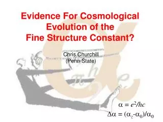
Cosmological Evolution of the Fine Structure Constant. a = e 2 /hc. Da = ( a z - a 0 )/ a 0. Chris Churchill (Penn State). In collaboration with: J. Webb, M. Murphy, V.V. Flambaum, V.A. Dzuba, J.D. Barrow, J.X. Prochaska, & A.M. Wolfe. Your “Walk Away” Info.

E N D
Cosmological Evolutionof the Fine Structure Constant a = e2/hc Da = (az-a0)/a0 Chris Churchill (Penn State) In collaboration with: J. Webb, M. Murphy, V.V. Flambaum, V.A. Dzuba, J.D. Barrow, J.X. Prochaska, & A.M. Wolfe
Your “Walk Away” Info • 49 absorption cloud systems over redshifts 0.5–3.5 toward 28 QSOs compared to lab wavelengths for many transitions • 2 different data sets; • low-z (Mg II, Mg I, Fe II) • high-z (Si II, Cr II, Zn II, Ni II, Al II, Al III) • Find Da/a = (–0.72±0.18) × 10-5 (4.1s) (statistical) • Most important systematic errors are atmospheric dispersion (differential stretching of spectra) and isotopic abundance evolution (Mg & Si; slight shifting in transition wavelengths) • Correction for systematic errors yields stronger a evolution
Executive Summary • History/Motivations • Terrestrial and CMB/BBN • QSO Absorption Line Method • Doublet Method (DM) & Results • Many-Multiplet Method (MM) & Results • Statistical and Systematic Concerns • Concluding Remarks
Classes of Theories • Multi-dimensional and String Theories • Scalar Theories (varying electron charge) • Varying Speed of Light Theories Unification of quantum gravity with other forces… Couples E+M to cosmological mass density… Attempts to solve some cosmological problems…
Varying Electron Charge Theories Variation occurs over matter dominated epoch of the universe. L r g (Barrow etal 2001)
Varying Speed of Light Theories Motivation is to solve the “flatness” and “horizon” problems of cosmology generated by inflation theory (Barrow 1999, Moffat 2001). Theory allows variation in a to be ~10-5H0 at redshift z=1. Evolution is proportional to ratio of radiation to matter density.
CMB Behavior and Constraints Smaller a delays epoch of last scattering and results in first peak at larger scales (smaller l) and suppressed second peak due to larger baryon to photon density ratio. Last scattering vs. z CMB spectrum vs. l Solid (da=0); Dashed (da=-0.05); dotted (da=+0.05) Battye etal (2000)
BBN Behavior and Constraints D, 3He, 4He, 7Li abundances depend upon baryon fraction, Wb. Changing a changes Wb by changing p-n mass difference and Coulomb barrier. Avelino etal claim no statistical significance for a changed a from neither the CMB nor BBN data. They refute the “cosmic concordance” results of Battye etal, who claim that da=-0.05 is favored by CMB data. Avelino etal (2001)
QSO Absorption Lines (history) QSO absorption line methods can sample huge time span Savedoff (1965) used doublet separations of emission lines from galaxies to search for a evolution (first cosmological setting) Bahcall, Sargent & Schmidt (1967) used alkali-doublet (AD) separations seen in absorption in QSO spectra.
And, of course… The Weapon. Keck Twins 10-meter Mirrors
2-Dimensional Echelle Image Dark features are absorption lines
Electron Energy and Atomic Configuration A change in a will lead to a change in the electron energy, D, according to where Z is the nuclear charge, |E| is the ionization potential, j and l are the total and orbital angular momentum, and C(l,j) is the contribution to the relativistic correction from the many body effect in many electron elements. Note proportion to Z2(heavy elements have larger change) Note change in sign as j increases and C(l,j) dominates
The “Doublet Method” ex. Mg IIll2796, 2803 Si IVll1393, 1402 A change in a will lead to a change in the doublet separation according to where (Dl/l)z and (Dl/l)0 are the relative separations at redshift z and in the lab, respectively. Dl 2796 2803
We model the complex profiles as multiple clouds, using Voigt profile fitting (Lorentzian + Gaussian convolved) Free parameters are redshift, z, and Da/a Lorentzian is natural line broadening Gaussian is thermal line broadening (line of sight)
Si IV Doublet Results: Da/a = –0.51.3 ×10-5 (Murphy et al 2001)
The “Many-Multiplet Method” The energy equation for a transition from the ground state at a redshift z, is written Ez = Ec + Q1Z2[R2-1] + K1(LS)Z2R2+ K2(LS)2Z4R4 Ec= energy of configuration center Q1, K1, K2 = relativistic coefficients L = electron total orbital angular momentum S = electron total spin R = az/a0 Z = nuclear charge
wz = w0 + q1x + q2y A convenient form is: wz= redshifted wave number w0 = rest-frame wave number q1, q2 = relativistic correction coefficients for Z and e- configuration x = (az/a0)2 - 1 y = (az/a0)4 - 1 Mg II 2803 Mg II 2796 Fe II 2600 Fe II 2586 Fe II 2382 Fe II 2374 Fe II 2344
w Shifts for Da/a ~ 10-5 Anchors & Data Precision A precision of Da/a ~ 10-5 requires uncertainties in w0 no greater than 0.03 cm-1 (~0.3 km s-1) Well suited to data quality… we can centroid lines to 0.6 km s-1, with precision going as 0.6/N½ km s-1 Typical accuracy is 0.002 cm-1, a systematic shift in these values would introduce only a Da/a ~ 10-6
Advantages/Strengths of the MM Method • Inclusion of all relativistic corrections, including ground states, provides an order of magnitude sensitivity gain over AD method • In principle, all transitions appearing in QSO absorption systems are fair game, providing a statistical gain for higher precision constraints on Da/a compared to AD method • Inclusion of transitions with wide range of line strengths provides greater constraints on velocity structure (cloud redshifts) • (very important) Allows comparison of transitions with positive and negative q1 coefficients, which allows check on and minimization of systematic effects
Possible Systematic Errors • Laboratory wavelength errors • Heliocentric velocity variation • Differential isotopic saturation • Isotopic abundance variation (Mg and Si) • Hyperfine structure effects (Al II and Al III) • Magnetic fields • Kinematic Effects • Wavelength mis-calibration • Air-vacuum wavelength conversion (high-z sample) • Temperature changes during observations • Line blending • Atmospheric dispersion effects • Instrumental profile variations
Isotopic Abundance Variations There are no observations of high redshift isotopic abundances, so there is no a priori information Focus on the “anchors” Observations of Mg (Gay & Lambert 2000) and theoretical estimates of Si in stars (Timmes & Clayton 1996) show a metallicity dependence We re-computed Da/a for entire range of isotopic abundances from zero to terrestrial. This provides a secure upper limit on the effect.
Correction for Isotopic Abundances Effect low-z Data Corrected Uncorrected This is because all Fe II are to blue of Mg II anchor and have same q1 sign (positive) Leads to positive Da/a For high-z data, Zn II and Cr II are To red of Si II and Ni II anchors and have opposite q1 signs
Atmospheric Dispersion Causes an effective stretching of the spectrumwhich mimics a non-zero Da/a a = pixel size [Å] , d = slit width arcsec/pix, Dψ = angular separation of l1 and l2 on slit, θ = angle of slit relative to zenith Blue feature will have a truncated blue wing! Red feature will have a truncated red wing! This is similar to instrumental profile distortion, effectively a stretching of the spectrum
Correction for Atmospheric Distortions Effect low-z Data Corrected Uncorrected This is because all Fe II are to blue of Mg II anchor and have same q1 sign (positive) Leads to positive Da/a For high-z data, Zn II and Cr II are To blue and red of Si II and Ni II anchors and have opposite q1 signs
Summary of MM Method • 49 absorption clouds systems over redshifts 0.5 to 3.5 toward 28 QSOs compared to lab wavelengths for many transitions • 2 different data sets; • low-z (Mg II, Mg I, Fe II) • high-z (Si II, Cr II, Zn II, Ni II, Al II, Al III) • Find Da/a = (–0.72±0.18) × 10-5 (4.1s) (statistical) • Most important systematic errors are atmospheric dispersion (differential stretching of spectra) and isotopic abundance evolution (Mg & Si; slight shifting in transition wavelengths) • Correction for systematic errors yields stronger a evolution
Soon to the Press Preliminary Findings… Now have a grand total of 138 systems due to adding the HIRES data of Sargent et al. Find Da/a = (–0.65±0.11) × 10-5 (6s) (statistical) What We Need: The Future Same and new systems observed with different instrument and reduced/analyzed by different software and people. Our plans are to get UVES/VLT and HRS/HET spectra in order to reproduce the HIRES/Keck results