• URL: .../publications/courses/ece_8423/lectures/current/lecture_09

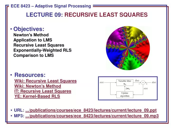
1. LECTURE 09: RECURSIVE LEAST SQUARES • Objectives:Newton’s MethodApplication to LMSRecursive Least SquaresExponentially-Weighted RLSComparison to LMS • Resources:Wiki: Recursive Least SquaresWiki: Newton’s MethodIT: Recursive Least SquaresYE: Kernel-Based RLS • URL: .../publications/courses/ece_8423/lectures/current/lecture_09.ppt • MP3: .../publications/courses/ece_8423/lectures/current/lecture_09.mp3

2. Newton’s Method • The main challenge with the steepest descent approach of the LMS algorithm is its slow and non-uniform convergence. • Another concern is the use of a single, instantaneous point estimate of the gradient (and we discussed an alternative block estimation approach). • We can derive a more powerful iterative approach that uses all previous data and is based on Newton’s method for finding the zeroes of a function. • Consider a function having a single zero: • Start with an initial guess, x0. • The next estimate is obtained byprojecting the tangent to the curve towhere it crosses the x-axis: • The next estimate is formed as x1, andgeneral iterative formula is:

3. Application to Adaptive Filtering • To apply this to the problem of least-squares minimization, we must find the zero of the gradient of the mean-squared error. • Since the mean-squared error is a quadratic function, the gradient is linear, and hence convergence takes place in a single step. • Noting that , recall our error function: • We find the optimal solution by equating the gradient of the error to zero: • and the optimum solution is: • We can demonstrate that the Newton algorithm is given by: • by substituting our expression for the gradient: • Note that this still requires an estimate of the autocorrelation and derivative.

4. Estimating the Gradient • In practice, we can use an estimate of the gradient, , as we did for the LMS gradient. The update equation becomes: • The noisy estimate of the gradient will produce excess mean-squared error. To combat this, we can introduce an adaptation constant: • Of course, convergence no longer occurs in one step, and we are somewhat back to where we started with the iterative LMS algorithm, and we have to worry about estimation the autocorrelation matrix. • To compare this solution to the LMS algorithm, we can rewrite the update equation in terms of the error signal: • Taking the expectation of both sides, and invoking independence: • Note that if  = 1: . Our solution is simply a weighted average of the previous value and newest estimate.

5. Analysis of Convergence • Once again we can define an error vector: • The solution to this first-order difference equation is: • We can observe the following: • The algorithm converges in the mean provided: • Convergence proceeds exponentially at a rate determined by . • The convergence rate of each coefficient is identical and independent of the eigenvalue spread of the autocorrelation matrix, R. • The last point is a crucial difference between the Newton algorithm and LMS. • We still need to worry about our estimate of the autocorrelation matrix, R: • and we assume x(n) = 0 for n < 0. We can write an update equation as a function of n:

6. Estimation of the Autocorrelation Matrix and Its Inverse • The effort to estimate the autocorrelation matrix and its inverse is still considerable. We can easily derive an update equation for the autocorrelation: • To reduce the computational complexity of the inverse, we can invoke the matrix inversion lemma: • Applying this to the update equation for the autocorrelation function: • Note that no matrix inversions are required ( is a scalar). • The computation is proportional to L2 rather than L3 for the inverse. • The autocorrelation is never calculated; its estimate is simple updated.

7. Summary of the Overall Algorithm Initialize Iterate for n = 0, 1, … There are a few approaches to the initialization in step (1). The most straightforward thing to do is: where the 2 is chosen to be a small positive constant (and can often be estimated based on a priori knowledge of the environment). This approach has been superseded by recursive-in-time least squares solutions, which we will study next.

8. Recursive Least Squares (RLS) • Consider minimization of a finite duration version of the error: • The objective of the RLS algorithm is to maintain a solution which is optimal at each iteration. Differentiation of the error leads to the normal equation: • Note that we can now write recursive-in-time equations for R and g: • We seek solutions of the form: • We can apply the matrix inversion lemma for computation of the inverse:

9. Recursive Least Squares (Cont.) • Define an intermediate vector variable, : • Define another intermediate scalar variable, : • Define the a priori error as: • reflecting that this is the error obtained using the old filter and the new data. • Using this definition, we can rewrite the RLS algorithm update equation as:

10. Summary of the RLS Algorithm • Initialize • Iterate for n = 0, 1, … • Compare this to the Newton method: • The RLS algorithm can be expected to converge more quickly because the use of an aggressive, adaptive step size.

11. Exponentially-Weighted RLS Algorithm • We can define a weighted error function: • This gives more weight to the most recent errors. • The RLS algorithm can be modified in this case: • Initialize • Iterate for n = 1, 2, … • RLS is computationally more complex than simple LMS because it is O(L2). • In principle, convergence is independent of the eigenvalue structure of the signal due to the premultiplication by the inverse of the autocorrelation matrix.

12. Example: LMS and RLS Comparison • An IID sequence, x(n), is input to a filter: • Measurement noise was assumed to be zero-mean Gaussian noise with unit variance, and a gain such that the SNR was 40 dB. • The norm of the coefficient error vector is plotted in the top figure for 1000 trials. • The filter length, L, was set to 8; the LMS adaptation constant, , was set to 0.05. • The adaptation step-size was set to the largest value for which the LMS algorithm would give stable results, and yet the RLS algorithm still outperforms LMS. • The lower figure corresponds to the same analysis with an input sequence: • Why is performance in this case degraded?

13. Summary • Introduced Newton’s method as an alternative to simple LMS. • Derived the update equations for this approach. • Introduced the Recursive Least Squares (RLS) approach and an exponentially-weighted version of RLS. • Briefly discussed convergence and computational complexity. • Next: IIR adaptive filters.