Download
1 / 58
580 likes | 708 Views
LING 696B: Mixture model and linear dimension reduction. Statistical estimation. Basic setup: The world: distributions p(x; ), -- parameters “all models may be wrong, but some are useful”

E N D
Statistical estimation • Basic setup: • The world: distributions p(x; ), -- parameters “all models may be wrong, but some are useful” • Given parameter , p(x; ) tells us how to calculate the probability of x (also referred to as the “likelihood” p(x|) ) • Observations: X = {x1, x2, …, xN} generated from some p(x; ). N is the number of observations • Model-fitting: based on some examples X, make guesses (learning, inference) about
Statistical estimation • Example: • Assuming people’s height follows normal distributions (mean, var) • p(x; ) = the probability density function of normal distribution • Observation: measurements of people’s height • Goal: estimate parameters of the normal distribution
Maximum likelihood estimate (MLE) • Likelihood function: examples xi are independent of one another, so • Among all the possible values of , choose the so that L() is the biggest Consistency: L() H !
H matters a lot! • Example: curve fitting with polynomials
Clustering • Need to divide x1, x2, …, xN into clusters, without a priori knowledge of where clusters are • An unsupervised learning problem: fitting a mixture model to x1, x2, …, xN • Example: height of male and female follow two distributions, but don’t know gender from x1, x2, …, xN
The K-means algorithm • Start with a random assignment, calculate the means
The K-means algorithm • Re-assign members to the closest cluster according to the means
The K-means algorithm • Update the means based on the new assignments, and iterate
Why does K-means work? • In the beginning, the centers are poorly chosen, so the clusters overlap a lot • But if centers are moving away from each other, then clusters tend to separate better • Vice versa, if clusters are well-separated, then the centers will stay away from each other • Intuitively, these two steps “help each other”
Interpreting K-means as statistical estimation • Equivalent to fitting a mixture of Gaussians with: • Spherical covariance • Uniform prior (weights on each Gaussian) • Problems: • Ambiguous data should have gradient membership • Shape of the clusters may not be spherical • Size of the cluster should play a role
Multivariate Gaussian • 1-D: N(, 2) • N-D: N(, ), ~NX1 vector, ~NXN matrix with (i,j) = ij ~ correlation • Probability calculation: • P(x; ,) = C ||-N/2 exp{-(x-)T -1 (x-)} • Intuitive meaning of -1: how to calculate the distance from x to transpose inverse
Multivariate Gaussian: log likelihood and distance • Spherical covariance matrix -1 • Diagonal covariance matrix -1 • Full covariance matrix -1
Learning mixture of Gaussian:EM algorithm • Expectation: putting “soft” labels on data -- a pair (, 1-) (0.05, 0.95) (0.8, 0.2) (0.5, 0.5)
Learning mixture of Gaussian:EM algorithm • Maximization: doing Maximum-Likelihood with weighted data Notice everyone is wearing a hat!
EM v.s. K-means • Same: • Iterative optimization, provably converge (see demo) • EM better captures the intuition: • Ambiguous data are assigned gradient membership • Clusters can be arbitrary shaped pancakes • Size of the cluster is a parameter • Allows for flexible control based on prior knowledge (see demo)
EM is everywhere • Our problem: the labels are important, yet not observable – “hidden variables” • This situation is common for complex models, and Maximum likelihood --> EM • Bayesian Networks • Hidden Markov models • Probabilistic Context Free Grammars • Linear Dynamic Systems
Beyond Maximum likelihood?Statistical parsing • Interesting remark from Mark Johnson: • Intialize a PCFG with treebank counts • Train the PCFG on treebank with EM • A large a mount of NLP research try to dump the first, and improve the second Measure of success Log likelihood
What’s wrong with this? • Mark Johnson’s idea: • Wrong data: human don’t just learn from strings • Wrong model: human syntax isn’t context-free • Wrong way of calculating likelihood: p(sentence | PCFG) isn’t informative • (Maybe) wrong measure of success?
End of excursion:Mixture of many things • Any generative model can be combined with a mixture model to deal with categorical data • Examples: • Mixture of Gaussians • Mixture of HMMs • Mixture of Factor Analyzers • Mixture of Expert networks • It all depends on what you are modeling
Applying to the speech domain • Speech signals have high dimensions • Using front-end acoustic modeling from speech recognition: Mel-Frequency Cepstral Coefficients (MFCC) • Speech sounds are dynamic • Dynamic acoustic modeling: MFCC-delta • Mixture components are Hidden Markov Models (HMM)
Clustering speech with K-means • Phones from TIMIT
Clustering speech with K-means • Diphones • Words
What’s wrong here • Longer sound sequences are more distinguishable for people • Yet doing K-means on static feature vectors misses the change over time • Mixture components must be able to capture dynamic data • Solution: mixture of HMMs
HMM Mixture burst Mixture of HMMs • HMM silence transition • Learning: EM for HMM + EM for mixture
HMM mixture for whole sequences Gaussian mixture for single frames Mixture of HMMs • Model-based clustering • Front-end (MFCC+delta) • Algorithm: initial guess by K-means, then EM
Mixture of HMM v.s. K-means • Phone clustering: 7 phones from 22 speakers *1 – 5: cluster index
Mixture of HMM v.s. K-means • Diphone clustering: 6 diphones from 300+ speakers
Mixture of HMM v.s. K-means • Word clustering: 3 words from 300+ speakers
Growing the model • Guess 6 at once is hard, but 2 is easy; • Hill climbing strategy: starting with 2, then 3, 4, ... • Implementation: split the cluster with the maximum gain in likelihood; • Intuition: discriminate within the biggest pile.
1 2 11 12 21 22 Learning categories and features with mixture model • Procedure: apply mixture model and EM algorithm, inductively find clusters • Each split is followed by a retraining step using all data Data
% classified as Cluster 1 IPA TIMIT All data T D 1 obstruent 2 sonorant R ? R) j l % classified as Cluster 2
% classifed as Cluster 11 All data S 1 1 2 tS T d D 11 fricative 12 % classified as Cluster 12
% classified as Cluster 21 l All data u r 1 1 2 oU R oI A AU 11 12 21 backsonorant 22 aI U u I i eI i j % classified as Cluster 22
% classified Cluster 121 All data 1 1 2 11 12 21 22 121 oralstop 122nasalstop % classified as Cluster 122
back sonorant fricative oral stop nasal front low sonorant front high sonorant % classified as Cluster 221 All data j i 1 1 2 I 11 12 21 22 eI 121 122 221 222 % classified as Cluster 222
[- sonorant] 1 [+sonorant] [+fricative] [-fricative] [+back] [-back] [-nasal] [+nasal] [+high] [-high] Summary: learning features • Discovered features: distinctions between natural classes based on spectral properties All data • For individual sounds, the feature values are gradient rather than binary (Ladefoged, 01)
Evaluation: phone classification • How do the “soft” classes fit into “hard” ones? Training set Test set Are “errors” really errors?
Level 2: Learning segments + phonotactics • Segmentation is a kind of hidden structure • Iterative strategy works here too • Optimization -- the augmented model:p(words | units, phonotactics, segmentation) • Units argmax p({wi} | U, P, {si})Clustering = argmax p(segments | units) -- Level 1 • Phonotactics argmax p({wi} | U, P, {si})Estimating transitions of Markov chain • Segmentation argmax p({wi} | U, P, {si})Viterbi decoding
Iterative learning as coordinate-wise ascent Level curves of likelihood score Units phonotactics Initial value comes from Level-1 learning segmentation • Each step increases likelihood score and eventually reaches a local maximum
Level 3:Lexicon can be mixtures too • Re-clustering of words using the mixture-based lexical model • Initial values (mixture components, weights) bottom-up learning (Stage 2) • Iterating steps: • Classify each word as the best exemplar of the given lexical item (also infer segmentation) • Update lexical weights + units + phonotactics
Big question:How to choose K? • Basic problem: • Nested hypothesis spaces: Hk-1 Hk Hk+1 … • As K goes up, likelihood always goes up. • Recall the polynomial curve fitting • Mixture model too(see demo)
Big question:How to choose K? • Idea #1: don’t just look at the likelihood, look at the combination of likelihood and something else • Bayesian Information Criterion: -2 log L() + (log N)*d • Minimal Description Length:log L() + description() • Akaike Information Criterion: -2 log L() + 2 d/N • In practice, often need magical “weights” in front of the something else
Big question:How to choose K? • Idea #2: use one set of data for learning, one for testing generalization • Cross-validation: run EM until the likelihood starts to hurt in the test set (see demo) • What if you have a bad test set: Jack-knife procedure • Cutting data into 10 parts, and do 10 training and tests
Big question:How to choose K? • Idea #3: treat K as “hyper” parameter, and do Bayesian learning on K • More flexible: K can grow up and down depending on number of data • Allow K to grow to infinity: Dirichlet / Chinese restaurant process mixture • Need “hyper-hyper” parameters to control how likely K grows • Computationally also intensive
Big question:How to choose K? • There is really no elegant universal solution • One view: statistical learning looks within Hk, but does not come up with Hk itself • How do people choose K? (also see later reading)
Dimension reduction • Why dimension reduction? • Example: estimate a continuous probability distribution by counting histograms on samples 20 bins 30 bins 10 bins
Dimension reduction • Now think about 2D, 3D … • How many bins do you need? • Estimate density of distribution with Parzen window: • How big (r) does the window needs to grow? Data in the window Window size
Curse of dimensionality • Discrete distributions: • Phonetics experiment: M speakers X N sentences X P stresses X Q segments … … • Decision rules: (K) Nearest-neighbor • How big a K is safe? • How long do you have to wait until you are really sure they are your nearest neighbors?
One obvious solution • Assume we know something about the distribution • Translates to a parametric approach • Example: counting histograms for 10-D data needs lots of bins, but knowing it’s a pancake allows us to fit a Gaussian • d10 parameters v.s. how many?