Download
1 / 1
10 likes | 122 Views
Black : PDE Solution. Red : Monte Carlo Simulation. Continuum Models of Large Networks. G. Yang Zhang and Edwin K. P. Chong Joint work with Jan Hannig (University of North Carolina) and Don Estep (Colorado State University). P r. P l. Motivation

E N D
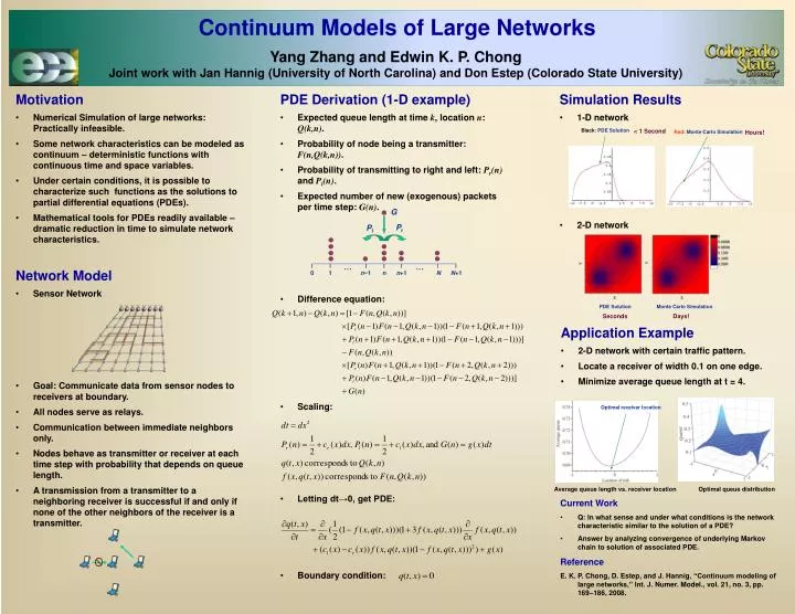
Black: PDE Solution Red: Monte Carlo Simulation Continuum Models of Large Networks G Yang Zhang and Edwin K. P. Chong Joint work with Jan Hannig(University of North Carolina) and Don Estep (Colorado State University) Pr Pl • Motivation • Numerical Simulation of large networks: Practically infeasible. • Some network characteristics can be modeled as continuum – deterministic functions with continuous time and space variables. • Under certain conditions, it is possible to characterize such functions as the solutions to partial differential equations (PDEs). • Mathematical tools for PDEs readily available – dramatic reduction in time to simulate network characteristics. • PDE Derivation (1-D example) • Expected queue length at time k, location n: Q(k,n). • Probability of node being a transmitter: F(n,Q(k,n)). • Probability of transmitting to right and left: Pr(n)and Pl(n). • Expected number of new (exogenous) packets per time step: G(n). • Difference equation: • Scaling: • Letting dt→0, get PDE: • Boundary condition: • Simulation Results • 1-D network • 2-D network … … 0 1 n−1 n n+1 N N+1 < 1 Second Hours! • Network Model • Sensor Network • Goal: Communicate data from sensor nodes to receivers at boundary. • All nodes serve as relays. • Communication between immediate neighbors only. • Nodes behave as transmitter or receiver at each time step with probability that depends on queue length. • A transmission from a transmitter to a neighboring receiver is successful if and only if none of the other neighbors of the receiver is a transmitter. PDE Solution Monte Carlo Simulation Seconds Days! • Application Example • 2-D network with certain traffic pattern. • Locate a receiver of width 0.1 on one edge. • Minimize average queue length at t = 4. Optimal receiver location Average queue length vs. receiver location Optimal queue distribution • Current Work • Q: In what sense and under what conditions is the network characteristic similar to the solution of a PDE? • Answer by analyzing convergence of underlying Markov chain to solution of associated PDE. Reference E. K. P. Chong, D. Estep, and J. Hannig, “Continuum modeling of large networks,” Int. J. Numer. Model., vol. 21, no. 3, pp. 169–186, 2008.