Download
1 / 44
440 likes | 645 Views
3. Vertical Data First, a brief description of Data Warehouses versus Database Management Systems. C.J. Date recommended, circa 1980, Do transaction processing on a DataBase Management System ( DBMS), rather than doing file processing on file systems .

E N D
3. Vertical DataFirst, a brief description of Data Warehouses versus Database Management Systems • C.J. Date recommended, circa 1980, • Do transaction processing on a DataBase Management System (DBMS), rather than doing file processing on file systems. • “Using a DBMS, instead of file systems, • unifies data resources, • centralizes control, • standardizes usages, • minimizes redundancy and inconsistency, • maximizes data value and usage, • yadda, yadda, yadda...” • Inmon, et all, circa 1990 • “Buy a separate Data Warehouse for long-running queries and data mining” (separate from DBMS for transaction processing)”. • “Double your hardware! Double your software! Double your fun!
Data Warehouses (DWs)vs.DataBase Management Systems (DBMSs) • What happened? • Inmon's idea was a great marketing success!, • but fortold a great Concurrency Control Research & Development (CC R&D) failure! CC R&D people had failed to integrate transaction and query processing, Also Known As (AKA) OnLine Transaction Processing (OLTP) and OnLine Analytic Processing (OLAP), that is, update and read workloads) in one system with acceptable performance! • Marketing of Data Warehouses was so successful, nobody noticed the failure! (or seem to mind paying double ;-( • Most enterprises now have a separate DW from their DBMS
Some still hope that DWs and DBs will one day be unified again. The industry may demand it eventually; e.g., Already, there is research work on real time updating of DWs For now let’s just focus on DATA. You run up against two curses immediately in data processing. Curse of cardinality: solutions don’t scale well with respect to record volume. "files are too deep!" Curse of dimensionality:solutions don’t scale with respect to attribute dimension. "files are too wide!" • Curse of cardinality is a problem in the horizontal and vertical world! • In the horizontal world it was disguised as “curse of the slow join”. In the horizontal world we decompose relations to get good design (e.g., 3rd normal form), but then we pay for that by requiring many slow joins to get the answers we need.
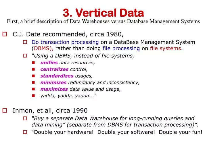
Techniques to address these curses. Horizontal processing of vertical data (instead of the ubiquitous vertical processing of horizontal (record orientated) data. Parallelizing the processing engine. • Parallelize the software engine on clusters of computers. • Parallelize the greyware engine on clusters of people (i.e., enable visualization and use the web...). Why do we need better techniques for data analysis, querying and mining? Data volume expands by Parkinson’s Law: Data volume expands to fill available data storage. Disk-storage expands by Moore’s law: Available storage doubles every 9 months!
Grasshopper caused significant economic loss each year. TIFF image Yield Map Early infestation prediction is key to damage control. A few successes: 1. Precision Agriculture Yield prediction:dataset consists of an aerial photograph (RGB TIFF image taken during the growing season) and a synchronized yield map (crop yield taken at harvest); thus, 4 feature attributes (B,G,R,Y) and ~100,000 pixels Producer are able to analyze the color intensity patterns from aerial and satellite photos taken in mid season to predict yield (find associations between electromagnetic reflection and yeild). One is ”hi_green&low_red hi_yield”. That is very intuitive. A stronger association was found strictly by data mining: “hi_NIR & low_redhi_yield” Once found in historical data (through data mining), producers just query TIFF images mid-season for low_NIR & high_red grid cells. Where low yeild is predicted, they then apply additional nitrogen. Can producers use Landsat images of China of predict wheat prices before planting? Grasshopper Infestation Prediction (again involving RSI data) Pixel classification on remotely sensed imagery holds significant promise to achieve early detection. Pixel classification (signaturing) has many apps: pest detection, fire detection, wet-lands monitoring … (for signaturing we developed the SMILEY software/greyware system) http:midas.cs.ndsu.nodak.edu/~smiley
2. Sensor Network Data • Micro and Nano scale sensor blocks are being developed for sensing • Biological agents • Chemical agents • Motion detection • coatings deterioration • RF-tagging of inventory (RFID tags for Supply Chain Mgmt) • Structural materials fatigue • There will be trillions++ of individual sensors creating mountains of data.
Situation space ================================== \ CARRIER / 2. A Sensor Network Application: CubE for Active Situation Replication (CEASR) Nano-sensors dropped into the Situation space Wherever threshold level is sensed (chem, bio, thermal...) a ping is registered in a compressed structure (P-tree – detailed definition coming up) for that location. Using Alien Technology’s Fluidic Self-assembly (FSA) technology, clear plexiglass laminates are joined into a cube, with a embedded nano-LED at each voxel. .:.:.:.:..::….:. : …:…:: ..: . . :: :.:…: :..:..::. .:: ..:.::.. .:.:.:.:..::….:. : …:…:: ..: . . :: :.:…: :..:..::. .:: ..:.::.. .:.:.:.:..::….:. : …:…:: ..: . . :: :.:…: :..:..::. .:: ..:.::.. The single compressed structure (P-tree) containing all the information is transmitted to the cube, where the pattern is reconstructed (uncompress, display). Each energized nano-sensor transmits a ping (location is triangulated from the ping). These locations are then translated to 3-dimensional coordinates at the display. The corresponding voxel on the display lights up. This is the expendable, one-time, cheap sensor version. A more sophisticated CEASR device could sense and transmit the intensity levels, lighting up the display voxel with the same intensity. Soldier sees replica of sensed situation prior to entering space
3. Anthropology ApplicationDigital Archive Network for Anthropology (DANA)(analyze, query and mine arthropological artifacts (shape, color, discovery location,…)
visualization Pattern Evaluation and Assay Data Mining Classification Clustering Rule Mining Loop backs Task-relevant Data Data Warehouse: cleaned, integrated, read-only, periodic, historical database Selection Feature extraction, tuple selection Raw data must be cleaned of: missing items, outliers, noise, errors Smart files What has spawned these successes?(i.e., What is Data Mining?) Queryingis asking specific questions for specific answers Data Mining is finding the patterns that exist in data (going into MOUNTAINS of raw data for the information gems hidden in that mountain of data.)
Fractals, … Standard querying Searching and Aggregating Data Prospecting Machine Learning Data Mining Association Rule Mining OLAP (rollup, drilldown, slice/dice.. Supervised Learning – classification regression SQL SELECT FROM WHERE Complex queries (nested, EXISTS..) FUZZY query, Search engines, BLAST searches Unsupervised Learning - clustering Walmart vs.KMart Data Mining versus Querying There is a whole spectrum of techniques to get information from data: Even on the Query end, much work is yet to be done(D. DeWitt, ACM SIGMOD Record’02). On the Data Mining end, the surface has barely beenscratched. But even those scratches had a great impact – One of the early scatchers became the biggest corporation in the world. A Non-scratcher filed for bankruptcy protection. Our Approach:Vertical, compressed data structures, Predicate-trees or Peano-trees (Ptrees in either case)1 processed horizontally (DBMSs processhorizontal data vertically) • Ptrees are data-mining-ready, compressed data structures, which attempt to address the curses of scalability and curse of dimensionality. 1 Ptree Technology is patented by North Dakota State University
Predicate trees (Ptrees): vertically project each attribute, R[A1] R[A2] R[A3] R[A4] 010 111 110 001 011 111 110 000 010 110 101 001 010 111 101 111 011 010 001 100 010 010 001 101 111 000 001 100 111 000 001 100 010 111 110 001 011 111 110 000 010 110 101 001 010 111 101 111 011 010 001 100 010 010 001 101 111 000 001 100 111 000 001 100 for Horizontally structured records Scan vertically = pure1? true=1 pure1? false=0 R11 R12 R13 R21 R22 R23 R31 R32 R33 R41 R42 R43 0 1 0 1 1 1 1 1 0 0 0 1 0 1 1 1 1 1 1 1 0 0 0 0 0 1 0 1 1 0 1 0 1 0 0 1 0 1 0 1 1 1 1 0 1 1 1 1 0 1 1 0 1 0 0 0 1 1 0 0 0 1 0 0 1 0 0 0 1 1 0 1 1 1 1 0 0 0 0 0 1 1 0 0 1 1 1 0 0 0 0 0 1 1 0 0 pure1? false=0 pure1? false=0 pure1? false=0 0 0 0 1 0 01 0 1 0 1 0 1 1. Whole is pure1? false 0 P11 P12 P13 P21 P22 P23 P31 P32 P33 P41 P42 P43 2. Left half pure1? false 0 P11 0 0 0 0 1 01 3. Right half pure1? false 0 0 0 0 0 1 0 0 10 01 0 0 0 1 0 0 0 0 0 0 0 1 01 10 0 0 0 0 1 0 0 0 0 1 0 0 0 0 0 0 0 0 1 0 0 0 0 0 0 1 0 0 ^ ^ ^ ^ ^ ^ ^ 0 0 1 0 1 4. Left half of rt half? false0 0 0 1 0 1 01 5. Rt half of right half? true1 0 1 0 What are Ptrees? then vertically project each bit position of each attribute, Given a table structure into horizontal records. Process it (scan it) vertically then compress each bit slice into a basic Ptree. e.g., compression of R11 into P11 goes as follows: 2 (e.g., to find # of occurences of7 0 1 4 =?) R(A1 A2 A3 A4) Base 10 Base 2 2 7 6 1 6 7 6 0 3 7 5 1 2 7 5 7 3 2 1 4 2 2 1 5 7 0 1 4 7 0 1 4 R11 0 0 0 0 0 0 1 1 Top-down construction of the 1-dimensional Ptree of R11, denoted, P11: Record the truth of the universal predicate pure 1 in a tree recursively on halves (1/21 subsets), until purity is achieved. P11 But it is pure (pure0) so this branch ends To find # occurences of 7 0 1 4, horizontally AND basic Ptrees (next slide)
R[A1] R[A2] R[A3] R[A4] 010 111 110 001 011 111 110 000 010 110 101 001 010 111 101 111 101 010 001 100 010 010 001 101 111 000 001 100 111 000 001 100 010 111 110 001 011 111 110 000 010 110 101 001 010 111 101 111 101 010 001 100 010 010 001 101 111 000 001 100 111 000 001 100 = R11 R12 R13 R21 R22 R23 R31 R32 R33 R41 R42 R43 0 1 0 1 1 1 1 1 0 0 0 1 0 1 1 1 1 1 1 1 0 0 0 0 0 1 0 1 1 0 1 0 1 0 0 1 0 1 0 1 1 1 1 0 1 1 1 1 1 0 1 0 1 0 0 0 1 1 0 0 0 1 0 0 1 0 0 0 1 1 0 1 1 1 1 0 0 0 0 0 1 1 0 0 1 1 1 0 0 0 0 0 1 1 0 0 0 1 0 1 0 0 0 0 1 0 01 0 1 0 0 1 01 This 0 makes entire left branch 0 7 0 1 4 These 0s make this node 0 P11 P12 P13 P21 P22 P23 P31 P32 P33 P41 P42 P43 These 1s and these 0s make this 1 0 0 0 0 1 01 0 0 0 0 1 0 0 10 01 0 0 0 1 0 0 0 0 0 0 0 1 01 10 0 0 0 0 1 10 0 1 0 ^ ^ ^ ^ ^ ^ ^ ^ ^ 0 0 1 0 1 0 0 1 0 1 01 0 1 0 R(A1 A2 A3 A4) 2 7 6 1 3 7 6 0 2 7 5 1 2 7 5 7 5 2 1 4 2 2 1 5 7 0 1 4 7 0 1 4 # change To count occurrences of 7,0,1,4 use 111000001100: 0 P11^P12^P13^P’21^P’22^P’23^P’31^P’32^P33^P41^P’42^P’43 = 0 0 01 ^ 21-level has the only 1-bit so the 1-count = 1*21 = 2
R11 0 0 0 0 1 0 1 1 Top-down construction of basic P-trees is best for understanding, bottom-up is much faster (once across). 0 0 0 0 0 1 0 0 0 0 0 1 1 1 Bottom-up construction of 1-Dim, P11, is done using in-order tree traversal, collapsing of pure siblings as we go: P11 R11 R12 R13 R21 R22 R23 R31 R32 R33 R41 R42 R43 0 1 0 1 1 1 1 1 0 0 0 1 0 1 1 1 1 1 1 1 0 0 0 0 0 1 0 1 1 0 1 0 1 0 0 1 0 1 0 1 1 1 1 0 1 1 1 1 1 0 1 0 1 0 0 0 1 1 0 0 0 1 0 0 1 0 0 0 1 1 0 1 1 1 1 0 0 0 0 0 1 1 0 0 1 1 1 0 0 0 0 0 1 1 0 0 0
A Education Database Example Student Courses Enrollments C# CNAME ST TERM S# SNAME GEN C# S# GR In this example database (which is used throughout these notes), there are two entities, Students (a student has a number, S#, a name, SNAME, and gender, GEN Courses (course has a number, C#, name, CNAME, State where the course is offered, ST, TERM and ONE relationship, Enrollments (a student, S#, enrolls in a class, C#, and gets a grade in that class, GR). The horizontal Education Database consists of 3 files, each of which consists of a number of instances of identically structured horizontal records: Enrollments Student Courses S#|C#|GR 0 |1 |B 0 |0 |A 3 |1 |A 3 |3 |B 1 |3 |B 1 |0 |D 2 |2 |D 2 |3 |A 4 |4 |B 5 |5 |B S#|SNAME|GEN 0 |CLAY | M 1 |THAD | M 2 |QING | F 3 |AMAL | M 4 |BARB | F 5 |JOAN | F C#|CNAME|ST|TERM 0 |BI |ND| F 1 |DB |ND| S 2 |DM |NJ| S 3 |DS |ND| F 4 |SE |NJ| S 5 |AI |ND| F We have already talked about the process of structuring data in a horizontal database (e.g., develop an Entity-Relationship diagram or ER diagram, etc. - in this case: What is the process of structuring this data into a vertical database? To be honest, that is an open question. Much research is needed on that issue! (great term paper topics exist here!!!) We will discuss this a little more on the next slide.
One way to begin to vertically structure this data is: 1. Code some attributes in binary (shown in red italics to the right of each field value encoded).For numeric fields, we have used standard binary encoding. For gender, F=1 and M=0. For term, Fall=0, Spring=1. For grade, A=11, B=10, C=01, D=00 (which could be called GPAencoding?). We have also abreviated STUDENT to S, COURSE to C and ENROLLMENT to E. S:S#___|SNAME|GEN 0 000|CLAY |M 0 1 001|THAD |M 0 2 010|QING |F 1 3 011|BARB |F 1 4 100|AMAL |M 0 5 101|JOAN |F 1 C:C#___|CNAME|ST|TERM 0 000|BI |ND|F 0 1 001|DB |ND|S 1 2 010|DM |NJ|S 1 3 011|DS |ND|F 0 4 100|SE |NJ|S 1 5 101|AI |ND|F 0 E:S#___|C#___|GR . 0 000|1 001|B 10 0 000|0 000|A 11 3 011|1 001|A 11 3 011|3 011|D 00 1 001|3 011|D 00 1 001|0 000|B 10 2 010|2 010|B 10 2 010|3 011|A 11 4 100|4 100|B 10 5 101|5 101|B 10 The above encoding seem natural. But how did we decide which attributes are to be encoded and which are not? As a term paper topic, that would be one of the main issues to research Note, we have decided not to encode names (our rough reasoning (not researched) is that there would be little advantage and it would be difficult (e.g. if name is a CHAR(25) datatype, then in binary that's 25*8 = 200 bits!). Note that we have decided not to encode State. That may be a mistake! Especially in this case, since it would be so easy (only 2 States ever? so 1 bit), but more generally there could be 50 and that would mean at least 6 bits. 2. Another binary encoding scheme (which can be used for numeric and non-numeric fields) is value map or bitmap encoding. The concept is simple. For each possible value, a, in the domain of the attribute, A, we encode 1=true and 0=false for the predicate A=a. The resulting single bit column becomes a map where a 1 means that row has A-value = a and a 0 means that row or tuple has A-value which is not a. There is a wealth of existing research on bit encoding. There is also quite a bit of research on vertical databases. There is even the first commercial vertical database announced called Vertica (check it out by Googling that name). Vertica was created by the same guy, Mike Stonebraker, who created one of the first Relational Databases, Ingres.
Way-1 for vertically structuring the Educational Database The W1 VDBMS would then be stored as: The Vertical bit sliced (uncompressed P-trees - P for Predicate) attributes stored as: S.s2S.s1S.s0S.gC.c2C.c1C.c0C.tE.s2E.s1E.s0E.c2E.c1E.c0E.g1 E.g0 0 0 0 0 0 0 0 00 0 0 0 0 1 1 0 0 0 1 0 0 0 1 10 0 0 0 0 0 1 1 1 0 0 0 1 0 0 10 0 1 0 1 1 0 0 1 0 1 1 1 0 1 00 0 1 0 0 0 1 0 0 1 0 1 0 1 0 10 1 1 0 1 1 1 1 0 1 1 1 0 1 1 00 1 1 0 1 1 0 0 0 1 0 0 1 0 1 0 0 1 0 0 0 1 1 1 1 0 0 1 0 0 1 0 1 0 1 1 0 1 1 0 The Vertical (un-bit-sliced) attributes are stored: S.name C.nameC.st |CLAY ||BI | |ND| |THAD ||DB | |ND| |QING ||DM | |NJ| |BARB ||DS | |ND| |AMAL ||SE | |NJ| |JOAN ||AI | |ND| Before moving on to 2 dimesional data encoding (e.g., images), we show one query processing algorithm for VDBMSs. Much more on this comes later in section 9 of the course.
Vertical Query Processing (another great term paper research area - see the notes on Query Processing, section 9 for more details) decimal binary. In the EDUC database (Students, Courses, Enrollments), numeric attributes are represented vertically as P-trees (not compressed). Categorical attributes (non-numeric) are projected to a 1 column vertical file S:s ngen |0 000| |0| |1 001| |0| |2 100| |1| |3 111| |1| |4 010| |0| |5 011| |1| S.s2 0 0 1 1 0 0 S.s1 0 0 0 0 1 1 S.s0 0 1 0 1 0 1 S.g 1 1 0 0 1 0 E:s |grade |0 000 |B 10| |0 000 |A 11| |3 011 |A 11| |3 011 |D 00| |1 001 |D 00| |1 001 |B 10| |2 010 |B 10| |2 010 |A 11| |4 100 |B 10| |5 101 |B 10| E.s2 0 0 0 0 0 0 0 0 1 1 E.s1 0 0 1 1 0 0 1 1 0 0 E.s0 0 0 1 1 1 1 0 0 0 1 E.g1 1 1 1 0 0 1 1 1 1 1 E.g0 0 1 1 0 0 0 0 1 0 0 SELECTS.n, E.g FROMS, E WHERES.s=E.s&E.g=D
S.s2 0 0 1 1 0 0 S.s1 0 0 0 0 1 1 S.s0 0 1 0 1 0 1 S.g 1 1 0 0 1 0 For the selection mask,E.g=D we perform EM= E'.g1AND E'.g2 (want both bits to be zero). E.s2 0 0 0 0 0 0 0 0 1 1 E.s1 0 0 1 1 0 0 1 1 0 0 E.s0 0 0 1 1 1 1 0 0 0 1 E'.g1 0 0 0 1 1 0 0 0 0 0 E.g1 1 1 1 0 0 1 1 1 1 1 E'.g0 1 0 1 1 0 1 1 0 1 1 E.g0 0 1 0 0 1 0 0 1 0 0 C.c1 0 0 1 1 C.c1 0 1 0 1 C.r1 0 1 1 1 C.r2 1 1 1 0 EM 0 0 0 1 0 0 0 0 0 0 SELECTS.n, E.g FROMS, E WHERES.s=E.s&E.g=D
E.s2 0 0 0 0 0 0 0 0 0 0 E.s1 0 0 1 0 0 0 0 1 0 0 E.s0 0 0 1 0 0 0 0 0 0 0 EM 0 0 0 1 0 0 0 0 0 0 S’.s2 1 1 0 0 1 0 S.s2 0 0 0 0 0 0 S'.s1 1 1 1 1 0 1 S.s1 0 0 0 0 1 0 S.s0 0 1 0 0 0 0 S’.s0 1 0 0 0 1 0 S.n CLAY THAD GOOD BRAD PERY JOAN For the join, E.s=S.san indexed nested loop like method can be used. SM 1 0 0 0 0 0 Get 1st masked E.s value, 000b Mask S tuples: P’S.s2AND PS.s1AND P’S.s0 Get S.n-value(s), C, pair it with E.g-value(s), output concatenation, S.nE.g CLAY D NOTE: The cost of processing this query is almost independent of cardinality of the files (number of rows). So if there were 12,000 students and 100,000 enrollments, except for the extra cost of ANDing longer bit vectors (which is insignificant - AND is the fasted operation in any computer), the query would process very rapidly. This is because no scan is required. SELECTS.n, E.g FROMS, E WHERES.s=E.s&E.g=D
1 1 1 1 1 1 0 0 1 1 1 1 1 0 0 0 1 1 1 1 1 1 0 0 1 1 1 1 1 1 1 0 1 1 1 1 0 0 0 0 1 1 1 1 0 0 0 0 1 1 1 1 0 0 0 0 0 1 1 1 0 0 0 0 2-Dimensional P-trees:natural choice for, e.g., 2-D image files.For images, any ordering of pixels will work (raster, diagonalized, Peano, Hilbert, Jordan), but the space-filling “Peano” ordering has advantages for fast processing, yet compresses well in the presence of spatial continuity. For an image bit-file (e.g., hi-order bit of the red color band of an image): 1111110011111000111111001111111011110000111100001111000001110000 Which, in spatial raster order is: Top-down construction of its 2-dimensional Peano ordered P-tree is built by recording the truth of universal predicate “pure 1” in a fanout=4 tree recursively on quarters (1/22 subsets), until purity achieved Pure-1? False=0 Pure! Pure! 0 1 0 0 0 pure! pure! pure! pure! pure! 0 0 1 0 1 1 0 1 1 1 1 0 0 0 1 0 1 1 0 1
Start here 1 0 0 0 1 1 1 1 1 0 1 0 0 0 0 1 1 0 1 0 0 1 1 1 1 1 1 0 0 0 1 1 1 1 1 1 1 1 1 1 1 1 1 1 1 1 1 1 1 0 1 1 1 1 1 1 1 1 1 1 1 1 0 0 0 0 0 1 0 0 0 0 0 0 0 0 0 0 0 0 0 0 0 0 1 1 1 1 1 1 0 0 1 1 1 1 1 0 0 0 1 1 1 1 1 1 0 0 1 1 1 1 1 1 1 0 1 1 1 1 0 0 0 0 1 1 1 1 0 0 0 0 1 1 1 1 0 0 0 0 0 1 1 1 0 0 0 0 Bottom-up construction of the 2-Dimensional P-tree is done using Peano (in order) traversal of a fanout=4, log4(64)= 4 level tree, collapsing pure siblings, as we go: From here on we will take 4 bit positions at a time, for efficiency.
1=001 0 level-3 (pure=43) 0 1 1 1 1 1 1 0 0 1 1 1 1 1 0 0 0 1 1 1 1 1 1 0 0 1 1 1 1 1 1 1 0 1 1 1 1 1 1 1 1 1 1 1 1 1 1 1 1 1 1 1 1 1 1 1 1 0 1 1 1 1 1 1 1 0 1 2 3 1 1 0 0 0 0 1 1 level-2 (pure=42) 2 0 0 0 0 1 1 0 0 0 1 1 0 0 0 1 1 level-1 (pure=41) 3 7=111 1 1 1 1 1 1 0 0 0 0 0 0 1 1 0 0 1 1 1 1 0 0 1 level-0 (pure=40) 1 2 . 2 . 3 ( 7, 1 ) 10.10.11 ( 111, 001 ) Some aspects of 2-D P-trees: ROOT-COUNT = level-sum * level-purity-factor. Root Count = 7 * 40 + 4 * 41 + 2 * 42 = 55 Node ID (NID) = 2.2.3 Tree levels (going down): 3, 2, 1, 0, with purity-factors of 43 42 41 40 respectively Fan-out = 2dimension = 22 = 4
3-Dimensional Ptrees:Top-down construction of its 3-dimensional Peano ordered P-tree: record the truth of universal predicate pure1 in a fanout=8 tree recursively on eighths (1/23 subsets), until purity achieved.Bottom-up construction of the 3-Dimensional P-tree is done using Peano (in order) traversal of a fanout=8, log8(64)= 2 level tree, collapsing pure siblings, as we go:
Suppose a biological agent is sensed by nano-sensors at a position in the situation space. And that position corresponds to this 1-bit position in this cutaway view Situation space We have now captured the data in the 1st octant (forward-upper-left). Moving to the next octant (forward-upper-right): 0 0 0 0 0 0 0 0 0 0 0 1 0 0 0 0 0 0 0 0 0 0 0 0 0 0 0 0 0 0 0 0 0 0 0 0 0 0 0 0 0 0 0 0 0 0 0 0 0 0 0 0 0 0 0 0 0 0 0 0 0 0 0 0 0 0 0 0 0 0 0 0 CEASR bio-agent detector (uses 3-D Ptrees) All other positions contain a 0-bit, i.e., the level of bio-agent detected by the nano-sensors in each of the other 63 cells isbelow a danger threshold. Start 0 1 ONE tiny, 3-D P-tree can represent this “bio-situation” completely. It is constructed (bottom up) as a fan-out=8, 3-D P-tree, as follows. P We can save time by noting that all the remaining 56 cells (in 7 other octants) contain all 0s. Each of the next 7 octants will produce eight 0s at the leaf level (8 pure-0 siblings), each of which will collapse to a 0 at level-1. So, proceeding an octant at a time (rather than a cell at a time): This entire situation can be transmitted to a personal display unit, as merely two bytes of data plus their two NIDs. For NID, use [level, global_level_offset] rather than [local_segment_offset,…local_segment_offset]. So assume every node not sent is all 0s, that in any 13-bit node segment sent (only need send “mixed” segments), the 1st 2 bits are the level, the next 3 bits are the global_level_offset within that level (i.e., 0..7), the final 8 bits are the node’s data, then the complete situation can be transmitted as these 13 bits: 010000000 0001 If 2n3 cells(n=2 above) situation it will take only log2(n) blue, 23n-3 green, 8 red bits So even if there are 283=224~16,000,000 cells, transmit merely 3+21+8=32 bits.
Basic Ptrees for a 7 column, 8 bit table e.g., P11, P12, … , P18, P21, …, P28, …, P71, …, P78 AND Target Attribute Target Bit Position Value Ptrees (predicate: quad is purely target value in target attribute) e.g., P1, 5 = P1, 101 = P11 AND P12’ AND P13 AND Target Attribute Target Value Tuple Ptrees (predicate: quad is purely target tuple) e.g., P(1, 2, 3) = P(001, 010, 111) = P1, 001 AND P2, 010 AND P3, 111 AND/OR Rectangle Ptrees (predicate: quad is purely in target rectangle (product of intervals) e.g., P([13],, [0.2]) = (P1,1 OR P1,2 OR P1,3) AND (P3,0 OR P3,1 OR P3,2) Basic, Value and Tuple Ptrees
R( A1 A2 A3 A4) 010 111 110 001 011 111 110 000 010 110 101 001 010 111 101 111 101 010 001 100 010 010 001 101 111 000 001 100 111 000 001 100 R11 R12 R13 R21 R22 R23 R31 R32 R33 R41 R42 R43 R11 R12 R13 R21 R22 R23 R31 R32 R33 R41 R42 R43 0 1 0 1 1 1 1 1 0 0 0 1 0 1 1 1 1 1 1 1 0 0 0 0 0 1 0 1 1 0 1 0 1 0 0 1 0 1 0 1 1 1 1 0 1 1 1 1 1 0 1 0 1 0 0 0 1 1 0 0 0 1 0 0 1 0 0 0 1 1 0 1 1 1 1 0 0 0 0 0 1 1 0 0 1 1 1 0 0 0 0 0 1 1 0 0 0 1 0 1 1 1 1 1 0 0 0 1 0 1 1 1 1 1 1 1 0 0 0 0 0 1 0 1 1 0 1 0 1 0 0 1 0 1 0 1 1 1 1 0 1 1 1 1 1 0 1 0 1 0 0 0 1 1 0 0 0 1 0 0 1 0 0 0 1 1 0 1 1 1 1 0 0 0 0 0 1 1 0 0 1 1 1 0 0 0 0 0 1 1 0 0 1 Horizontal Processing of Vertical Structuresfor Record-based Workloads • For record-based workloads (where the result is a set of records), changing the horizontal record structure and then having to reconstruct it, may introduce too much post processing? • For data mining workloads, the result is often a bit (Yes/No, True/False) or another unstructured result, where there is no reconstructive post processing?
But even for some standard SQL queries, vertical data may be faster (evaluating when this is true would be an excellent research project) • For example, the SQL query, • SELECT Count * FROM purchases WHERE price $4,000.00 AND 1000 sales 500. • The answer is the root-count of the P-tree resulting from ANDing the price-interval-P-tree, Pprice[4000,) and the sales-interval-P-tree, Psales[500,1000] .
YOUR DATA MINING YOUR DATA Data Integration Language DIL Ptree (Predicates) Query Language PQL DII (Data Integration Interface) DMI (Data Mining Interface) Data Repository lossless, compressed, distributed, vertically-structured database Architecture for the DataMIME™ System(DataMIMEtm = data mining, NO NOISE) (PDMS = P-tree Data Mining System) Internet
Decimal Binary Unsorted relation Generalized Raster and Peano Sorting: generalizes to any table with numeric attributes (not just images). Raster Sorting: Attributes 1st Bit position 2nd Peano Sorting: Bit position 1st Attributes 2nd
Unsorted Generalized Raster Generalized Peano crop adult spam function mushroom Generalize Peano Sorting KNN speed improvement (using 5 UCI Machine Learning Repository data sets) 120 100 80 Time in Seconds 60 40 20 0
Astronomy Application:(National Virtual Observatory data) What Ptree dimension and what ordering should be used for astronomical data?, where all bodies are assumed on surface of celestial sphere (shares equatorial plane with earth and has no specified radius) Hierarchical Triangle Mesh Tree (HTM-tree, seems to be the accepted standard) Peano Triangle Mesh Tree (PTM-tree) Peano Celestial Coordinate tree (RA=Recession Angle (longitudinal angle); dec=declination (latitude angle) PTM is similar to HTM used in the Sloan Digital Sky Survey project. In both: • Sphere is divided into triangles • Triangle sides are always great circle segments. • PTM differs from HTM in the way in which they are ordered?
1,2 1,2 1,3,3 1,1,2 1,0 1,3,0 1,1,1 1,0 1,1,0 1,1 1,3 1,3,2 1,1 1.1.3 1,3,1 1,3 The difference between HTM and PTM-trees is in the ordering. 1 1 Ordering of PTM-tree Ordering of HTM Why use a different ordering?
dec RA PTM Triangulation of the Celestial Sphere The following ordering produces a sphere-surface filling curve with good continuity characteristics, For each level. Traverse southern hemisphere in the revere direction (just the identical pattern pushed down instead of pulled up, arriving at the Southern neighbor of the start point. Traverse southern hemisphere in the revere direction (just the identical pattern pushed down instead of pulled up, arriving at the Southern neighbor of the start point. left Equilateral triangle (90o sector) bounded by longitudinal and equatorial line segments right right left turn Traverse the next level of triangulation, alternating again with left-turn, right-turn, left-turn, right-turn..
PTM-triangulation - Next Level LRLR RLRL LRLR RLRL LRLR RLRL LRLR RLRL LRLR RLRL LRLR RLRL LRLR RLRL LRLR RLRL
90o 0o -90o 0o 360o Z Z Z Z Z Z Z Z Z Z Z Z Z Z Z Z Z Z Z Z Z Z Z Z Z Z Z Z Z Z Z Z Z Z Z Z Z Z Z Z Z Z Z Z Z Z Z Z Z Z Z Z Z Z Z Z Z Z Z Z Z Z Z Z Z Z Z Z Z Z Z Z Z Z Z Z Z Z Z Z Z Z Z Z Z Z Z Z Z Z Z Z Z Z Z Z Z Z Z Z Z Z Z Z Z Z Z Z Z Z Z Z Z Z Z Z Z Z Z Z Z Z Z Z Z Z Z Z Z Z Z Z Z Z Z Z Z Z Z Z Z Z Z Z Z Z Z Z Z Z Z Z Z Z Z Z Z Z Z Z Z Z Z Z Z Z Z Z Z Z Z Z Z Z Z Z Z Z Z Z Z Z Z Z Z Z Z Z Z Z Z Z Z Z Z Z Z Z Z Z Z Z Z Z Z Z Z Z Z Z Z Z Z Z Z Z Z Z Z Z Z Z Z Z Z Z Z Z Z Z Z Z Z Z Z Z Z Z Z Z Z Z Z Z Z Z Z Z Z Z Z Z Z Z Z Z Z Z Z Z Z Z Z Z Z Z Z Z Z Z Z Z Z Z Z Z Z Z Z Z Z Z Z Z Z Z Z Z Z Z Z Z Z Z Z Z Z Z Z Z Z Z Z Z Z Z Z Z Z Z Z Z Z Z Z Z Z Z Z Z Z Z Z Z Z Z Z Z Z Z Z Z Z Z Z Z Z Z Z Z Z Z Z Z Z Z Z Z Z Z Z Z Z Z Z Z Z Z Z Z Z Z Z Z Z Z Z Z Z Z Z Z Z Z Z Z Z Z Z Z Z Z Z Z Z Z Z Z Z Z Z Z Z Z Z Z Z Z Z Z Z Z Z Z Z Z Z Z Z Z Z Z Z Z Z Z Z Z Z Z Z Z Z Z Z Z Z Z Z Z Z Z Z Z Z Z Z Z Z Z Z Z Z Z Z Z Z Z Z Z Z Z Z Z Z Z Z Z Z Z Z Z Z Z Z Z Z Z Z Z Z Z Z Z Z Z Z Z Z Z Z Z Z Z Z Z Z Z Z Z Z Z Z Z Z Z Z Z Z Z Z Z Z Z Z Z Z Z Z Z Z Z South Plane Plane Peano Celestial Coordinates Unlike PTM-trees which initially partition the sphere into the 8 faces of an octahedron, in the PCCtree scheme: Sphere is tranformed to a cylinder, then into a rectangle, then standard Peano ordering is used on the Celestial Coordinates. • Celestial Coordinates Recession Angle (RA) runs from 0 to 360o dand Declination Angle (dec) runs from -90o to 90o. Sphere Cylinder
SubCell-Location Myta Ribo Nucl Ribo 17, 78 12, 60 Mi, 40 1, 48 10, 75 0 0 7, 40 0 14, 65 0 0 16, 76 0 9, 45 1, 43 Function apop meio mito apop StopCodonDensity .1 .1 .1 .9 PolyA-Tail 1 1 0 0 Organism Species Vert Genome Size (million bp) Gene Dimension Table g0 g1 g2 g3 o0 human Homo sapiens 1 3000 Organism Dimension Table o1 fly Drosophila melanogaster 0 185 o2 1 1 1 1 1 0 0 1 0 1 0 0 1 0 1 1 o3 0 1 0 1 1 0 0 1 0 1 0 1 1 0 0 0 yeast Saccharomyces cerevisiae 0 12.1 e0 1 0 1 1 0 1 1 1 1 1 0 1 1 0 1 0 e0 mouse Mus musculus 1 3000 e1 e1 e2 e2 e3 LAB PI UNV STR CTY STZ ED AD S H M N e3 Experiment Dimension Table (MIAME) 3 2 a c h 1 2 2 b s h 0 2 4 a c a 1 2 4 a s a 1 PUBLIC (Ptree Unfied BioLogical InformtiCs Data Cube and Dimension Tables) Gene-OrganismDimension Table (chromosome,length) Gene-Experiment-Organism Cube (1 iff that gene from that organism expresses at a threshold level in that experiment.) many-to-many-to-many relationship
SubCell-Location Myta Ribo Nucl Ribo Function apop meio mito apop StopCodonDensity .1 .1 .1 .9 PolyA-Tail 1 1 0 0 Original Gene Dimension Table g0 g0 1 0 0 1 g1 0 1 1 g2 0 1 0 1 g3 1 0 g1 0 1 1 0 1 0 1 0 1 g2 1 0 0 0 1 0 0 g3 Myta Ribo Nuc l apop Me i o Mi to SCD 1 SCD 2 SCD 3 SCD 4 Poly-A G E N E 1 0 0 1 0 1 0 0 0 1 1 g0 0 1 0 0 1 0 0 0 0 1 1 g1 0 0 1 0 0 1 0 0 0 1 0 g2 0 1 0 1 0 0 1 0 0 1 0 g3 Boolean Gene Dimension Table (Binary) g3 g2 g1 g0 Protein-Protein Interaction Pyramid 0
Association of Computing Machinery KDD-Cup-02http://www.biostat.wisc.edu/~craven/kddcup/winners.html BIOINFORMATICS Task: Yeast Gene Regulation Prediction • There are now experimental methods that allow biologists to measure some aspect of cellular "activity" for thousands of genes or proteins at a time. A key problem that often arises in such experiments is in interpreting or annotating these thousands of measurements. This KDD Cup task focused on using data mining methods to capture the regularities of genes that are characterized by similar activity in a given high-throughput experiment. To facilitate objective evaluation, this task did not involve experiment interpretation or annotation directly, but instead it involved devising models that, when trained to classify the measurements of some instances (i.e. genes), can accurately predict the response of held aside test instances. • The training and test data came from recent experiments with a set ofS. cerevisiae (yeast) strains in which each strain is characterized by a single gene being knocked out. Each instance in the data set represents a single gene, and the target value for an instance is a discretized measurement of how active some (hidden) system in the cell is when this gene is knocked out. The goal of the task is to learn a model that can accurately predict these discretized values. Such a model would be helpful in understanding how various genes are related to the hidden system. • The best overall score (Kowalczyk) was 1.3217 (summed AROC for the two partitions). The best score for the "narrow" partition was 0.6837 (Denecke et al), and the best score for the "broad" partition was 0.6781 (Amal Perera, Bill Jockheck, Willy Valdivia Granda, Anne Denton, Pratap Kotala and William Perrizo, North Dakota State UniversityKDD Cup Pagehttp://www.acm.org/sigkdd/explorations/
Association of Computing Machinery KDD-Cup-02http://www.biostat.wisc.edu/~craven/kddcup/winners.html My Team
Association of Computing Machinery KDD-Cup-06http://www.cs.unm.edu/kdd_cup_2006http://www.cs.ndsu.nodak.edu/~datasurg/kddcup06/kdd6News.html MEDICAL INFORMATICS Task: Computer Aided Detection of Pulmonary Embolism Description of CAD systems: Over the last decade, Computer-Aided Detection (CAD) systems have moved from the sole realm of academic publications, to robust commercial systems that are used by physicians in their clinical practice to help detect early cancer from medical images. For example, CAD systems have been employed to automatically detect (potentially cancerous) breast masses and calcifications in X-ray images, detect lung nodules in lung CT (computed tomography) images, and detect polyps in colon CT images to name a few CAD applications. CAD applications lead to very interesting data mining problems. Typical CAD training data sets are large and extremely unbalanced between positive and negative classes. Often, fewer than 1% of the examples are true positives. When searching for descriptive features that can characterize the target medical structures, researchers often deploy a large set of experimental features, which consequently introduces irrelevant and redundant features. Labeling is often noisy as labels are created by expert physicians, in many cases without corresponding ground truth from biopsies or other independent confirmations. In order to achieve clinical acceptance, CAD systems have to meet extremely high performance thresholds to provide value to physicians in their day-to-day practice. Finally, in order to be sold commercially (at least in the United States), most CAD systems have to undergo a clinical trial (in almost exactly the same way as a new drug would). Typically, the CAD system must demonstrate a statistically significant improvement in clinical performance, when used, for example, by community physicians (without any special knowledge of machine learning) on as yet unseen cases – i.e., the sensitivity of physicians with CAD must be (significantly) above their performance without CAD, and without a corresponding marked increase in false positives (which may lead to unnecessary biopsies or expensive tests). In summary, very challenging machine learning and data mining tasks have arisen from CAD systems
Association of Computing Machinery KDD-Cup-06 http://www.cs.unm.edu/kdd_cup_2006http://www.cs.ndsu.nodak.edu/~datasurg/kddcup06/kdd6News.html Challenge of Pulmonary Emboli Detection: Pulmonary embolism (PE) is a condition that occurs when an artery in the lung becomes blocked. In most cases, the blockage is caused by one or more blood clots that travel to the lungs from another part of your body. While PE is not always fatal, it is nevertheless the third most common cause of death in the US, with at least 650,000 cases occurring annually.1 The clinical challenge, particularly in an Emergency Room scenario, is to correctly diagnose patients that have a PE, and then send them on to therapy. This, however, is not easy, as the primary symptom of PE is dysapnea (shortness of breath), which has a variety of causes, some of which are relatively benign, making it hard to separate out the critically ill patients suffering from PE. The two crucial clinical challenges for a physician, therefore, are to diagnose whether a patient is suffering from PE and to identify the location of the PE. Computed Tomography Angiography (CTA) has emerged as an accurate diagnostic tool for PE. However, each CTA study consists of hundreds of images, each representing one slice of the lung. Manual reading of these slices is laborious, time consuming and complicated by various PE look-alikes (false positives) including respiratory motion artifacts, flowrelated artifacts, streak artifacts, partial volume artifacts, stair step artifacts, lymph nodes, and vascular bifurcation, among many others. Additionally, when PE is diagnosed, medications are given to prevent further clots, but these medications can sometimes lead to subsequent hemorrhage and bleeding since the patient must stay on them for a number of weeks after the diagnosis. Thus, the physician must review each CAD output carefully for correctness in order to prevent overdiagnosis. Because of this, the CAD system must provide only a small number of false positives per patient scan. CAD system Goal: To automatically identify PE’s. In an almost universal paradigm for CAD algorithms, this problem is addressed by a 3 stage system: 1. Identification of candidate regions of interest (ROI) from a medical image, 2. Computation of descriptive features for each candidate, and 3. Classification of each candidate (in this case, whether it is a PE or not) based on its features. NPV Task: One of the most useful applications for CAD would be a system with very high (100%?) Negative Predictive Value. In other words, if the CAD system had zero positive candidates for a given patient, we would like to be very confident that the patient was indeed free from PE’s. In a very real sense, this would be the “Holy Grail” of a PE CAD system. The best NPV score was by Amal Perera, William Perrizo, North Dakota State University (twice as high as the next best score!) http://www.acm.org/sigs/sigkdd/explorations/issue.php?volume=8&issue=2&year=2006&month=12
Association of Computing Machinery KDD-Cup-06 Professor William Perrizo and his PhD student Amal Shehan Perera of the department of computer science at North Dakota State University (NDSU) won the KDD-Cup 2006 Knowledge Discovery and Data Mining competition which was held in conjunction with the ACM SIGKDD International Conference on Knowledge Discovery and Data Mining. The ACM KDD-Cup is the most rigorous annual competition in the field of data mining and machine learning. The competition is open to all academic institutes, industries as well as individuals from around the world. Since its inception in 1997, the KDD-Cup competition has presented practical and challenging data mining problems. Considerable number of researchers and practitioners participate in this annual contest. KDD-Cup datasets have become benchmarks for data mining research over the years. KDD-Cup 2006 was conducted between May and August 2006 by the Association for Computing Machinery(ACM) Special Interest Group on Knowledge Discovery and Data Mining (SIGKDD). This year’s contest was for a Computer-Aided Detection (CAD) system that could identify pulmonary embolisms, or blood clots, in the lung through examinations of the features from Computed Tomography (CT) images. A typical CT study consists of hundreds of images, each representing one slice of the lung. Manual reading of these slices is laborious, time consuming and complicated. It is also very important to be accurate in the prediction. NDSU team won the Negative Predictive Value (NPV) task of the competition, which was characterized by the organizers as the "Holy Grail" of Computer Aided Detection (CAD) of pulmonary embolisms. Siemens Medical Solutions provided dataset for the contest. Over 200 teams from around the world registered for the competition and 65 entries were submitted. This year's tasks were particularly challenging due to multiple instance learning, nonlinear cost functions, skewed class distributions, noisy class labels, and sparse data space. The NDSU team used a combined nearest neighbor and boundary classification with genetic algorithm parameter optimization. Dr. William Perrizo is a senior Professor in Computer Science at the North Dakota State University. He leads the Data Systems Users and Research Group (DataSURG) involved in innovative research on scalable data mining research using vertical data structures in the Computer Science Department at NDSU. DataSURG has been supported by NSF, NASA, DARPA, and GSA. Amal Shehan Perera is a lecturer at the Department of Computer Science and Engineering at the University of Moratuwa, Sri Lanka on study leave to complete his PhD at NDSU.
Network Security Application(Network security through Vertical Structured data) • Network layers do their own partitioning • Packets, frames, etc. (usually independent of any intrinsic data structuring – e.g., record structure) • Fragmentation/Reassembly, Segmentation/Reassembly • Data privacy is compromised when the horizontal (stream) message content is eavesdropped upon at the reassembled level (in network • A standard solution is to host-encrypt the horizontal structure so that any network reassembled message is meaningless. • Alt.: Vertically structure (decompose, partition) data (e.g., basic Ptrees). • Send one Ptree per packet • Send intra-message packets separately • Trick flow classifiers into thinking the multiple packets associated with a particular message are unrelated. • The message is only meaningful after destination demux-ing • Note: the only basic Ptree that holds actual information is the high-order bit Ptree. Therefore encrypt it! • There is a whole passel of killer ideas associated with the concept of using vertical structuring data within network transmission units • Active networking? (AND basic Ptrees (or just certain levels of) at active net nodes?)
Network Security Application Cont. • Vertically structure (decompose, partition) data (e.g., basic Ptrees). • Send one P-tree (vertical bit-slice per packet • Send basic P-tree slices (for a given attribute) one at a time starting with the low order bit slice. • Encrypt it using some agreed upon algorithm (and key) (requires key distribution) • But then steganographically embed the crypto alg identity and key structure for the next higher order bit into the ptree (as the carrier message). • Continue to do that for each higher order bit until you get to the highest order bit. Until it arrives and unless each crypto has been broken (in time to apply it to the next level) the message is un-decipherable.