Download
1 / 38

E N D
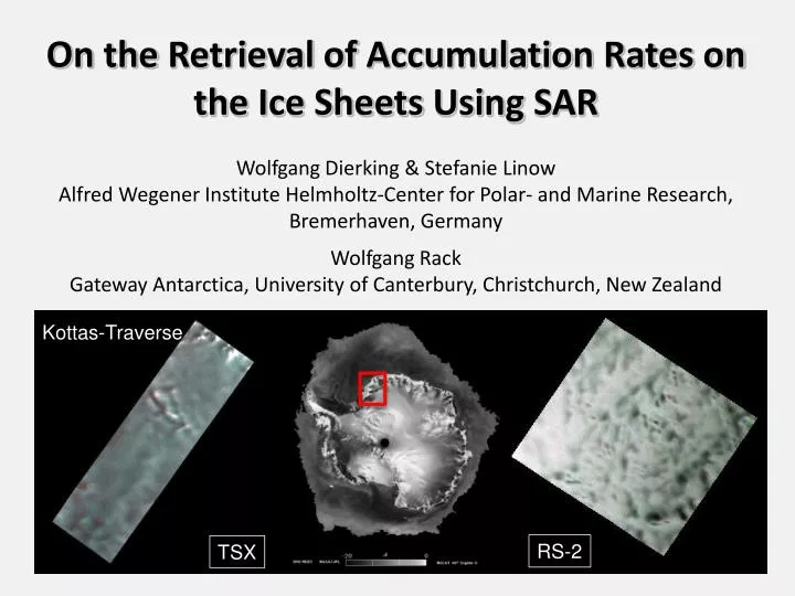
On theRetrievalofAccumulation Rates on theIce Sheets Using SAR Wolfgang Dierking & Stefanie LinowAlfred Wegener Institute Helmholtz-Center for Polar- and Marine Research, Bremerhaven, GermanyWolfgang RackGateway Antarctica, University of Canterbury, Christchurch, New Zealand Kottas-Traverse RS-2 TSX
Accumulation Rate Retrieval – Why? • Accumulation rates on • ice sheets: • do the ice sheets loose • mass? sea level rise • snow accumulation is • the gainin the mass • balance of an ice sheet Accumulation rates retrieved from AMSR-E 6.9 GHz satellite data combined with ground data (Arthern et al., JGR, 2006)
WhyUseRadar? Low accumulation rates: large grain sizes, thin annual layers Large accumulation rates: small grains, thicker layers • Radar (C to Ku-band) : • very sensitive to grain size • measured intensity depends on snow layering • high spatial resolution (SAR)
ExamplefromGreenland • Munk et al., JGR, 2003 • based on combination of snow metamorphosis and • radar scattering model • data: ERS-1 SAR • valid for dry-snow zone
ExamplefromGreenland Munk et al., JGR, 2003 Retrieved from SAR data In-situ data
Problems With Radar... • Large penetration depths • dependent on accumulation rate and temperature regime • C-band 20-80 m • Ku-band 5-20 m • (corresponding to covering 10s and up to 100s of years) • Is the backscattering coefficient sufficiently sensitive to • accumulation rate? • Different snow regimes – different sensitivities • (implications for snow metamorphosis model)
Sensitivityof σ0 toaccumulation rate Dierking et al., JGR, 2012
Snow Regimes FromScatterometry Rotschky et al., TGRS, Vol. 44, No. 4, 2006
Accumulation Versus σ0For Different Snow Regimes Rotschky et al., TGRS, Vol. 44, No. 4, 2006
Accumulation Rate Retrieval - Approach • Strategy: Combining • empirical models for snow parameter profiles (d, r, ρ) • (Linowet al., J. Glac., 2012) • radar scattering model asc desc From: Dierking et al., JGR 2012
Accumulation Rate Measurements Kottas Traverse: - stake measurements - 675 sites - 500 m intervals - down to 1.4-2 m depth asc desc From: Dierking et al., JGR 2012
Radar Scattering Model Radar scattering: volume contribution, regime bridging Scattering from firn: dense medium effect model (Wen et al., TGRS 1990) valid for firn densities < 0.3 g/cm3 (close-to-) surface firn density already 0.3-0.45 g/cm3 scatter regime bridging r, T fixed Dierking et al., JGR 2012
Radar Scattering Model scatter regime bridging …to be validated by numerical simulations or measurements… Qualitative agreement with scatterometer measurements by Kendra et al (1998) over artificial snow of density 0.5 g/cm3.
Model Results Versus Satellite SAR Data Comparison ModelledVs. Measured Sigma_Nought Envisat ASAR 2008/2009 low accumulation
Model Results Versus Satellite SAR Data Comparison ModelledVs. Measured Sigma_Nought Envisat ASAR 2008/2009 (wind) regime shift -> smaller snow crystals? low accumulation
Azimuthal Modulation of σ0 in Antarctica ERS-scatterometer C-Band • measured σ0 depends on sensor look direction • strong link with wind-generated surface undulations • - depends on incidence angle Long and Drinkwater, TGRS, 2000
ReasonForAzimuthalDependence? Surface undulations: sastrugi • high intensity if radar look direction perpendicular to crests • low intensity if radar look direction parallel to crests
Howto Model Surface/Interface Scattering? FromAshcraft & Long, J. Glac., Vol. 52, No. 177, 2006
Howto Model Surface/Interface Scattering? Small scale surface roughness: “Surface roughness parameters represent an equivalent single layer roughness estimate for a multi-layer surface” Depth hoar layers forming interfaces in the snow? Until now no convincing model exists for explaining the azimuthal variation of radar intensity… FromAshcraft & Long, J. Glac., Vol. 52, No. 177, 2006
New Data ForKottas Traverse • Multi-frequency, multi-polarization data: • additional information for model development • and accumulation rate retrieval ? • 6 RS-2 scenes from SOAR-EU, quad-pol. • January 2012 • 5 ascending, 1 descending • incidence angle 30.4-32°, pixel 25 m • 18 TSX scenes from MTH0123, SM HH+VV • February – April 2013 • 10 ascending, 8 descending • incidence angles 27.5-33.4, pixel 10 m
Spatial Distribution Intensity & Phase Radarsat-2 42,5 km 150 m 30.4-32° Backscattering Coefficient [dB] R – cross-pol., G-HH, B-VV Phase Difference HH-VV [rad] Kottas-Traverse, FQP 2012/01/24 72.76°S 9.53°W – 73.0°S 9.60°W
Spatial Distribution Intensity & Phase Radarsat-2 42,5 km 150 m 30.4-32° Undulations linked to topography? Yet no suffciently detailed DEM available for this area Backscattering Coefficient [dB] R – cross-pol., G-HH, B-VV Phase Difference HH-VV [rad] Kottas-Traverse, FQP 2012/01/24 72.76°S 9.53°W – 73.0°S 9.60°W
HistogramsCorrelation & Phase Radarsat-2 Phase Difference HH-VV [rad] Correlation Coefficient Kottas-Traverse, FQP 2012/01/24 72.76°S 9.53°W – 73.0°S 9.60°W
C-Band Radar Intensity Over Kottas-Traverse Radarsat-2 FQP data
Radar Intensity Versus Accumulation Rate Radarsat-2 72.2°S – 73.0°S T=-22 °C 73.0°S – 73.5°S T=-24°C
Radar Intensity Versus Accumulation Rate Radarsat-2 72.2°S – 73.0°S T=-22 °C Different snow regimes causing different sensitivities? 73.0°S – 73.5°S T=-24°C
Phase HH-VV vs. Accumulation Rate Radarsat-2
Phase HH-VV vs. Accumulation Rate Radarsat-2 • ???? • Azimuth slopes affect relative magnitude • and phase of all terms of the covariance • matrix (Lee et al., TGRS Vol. 38, No 5, 2000 • Anisotropic propagation in the firn? Preferred • orientation of snow crystals (wind compaction)? • But why related to accumulation rate?
X-Band Radar Intensity Over Kottas-Traverse TerraSAR-X SM Dual-Pol. difference asc - desc percolation zone
DifferenceAscending – Descending (C-Band) Envisat ASAR HH-polarization
Radar Intensity Versus AccumulationRate TerraSAR-X 72.2°S – 73.0°S T=-22 °C 73.0°S – 73.7°S T=-24 °C
Phase HH-VV vs. AccumulationRate TerraSAR-X
Summary Results from RS-2 and TSX-images • Sensitivitytoaccumulation rate: • Snow-regime dependent ? • C-band: cross-pol more sensitive thanlike-pol. • C- and X-band like-pol comparable • - Azimuthalmodulation: • Different between X- and C-band • - Phase difference HH-VV: changeasfunctionof • accumulation rate issignificantat C-band, • but not at X-band.
Problems • Noisydata! Problem for robust retrieval. • Issensitivityofσ0toaccumulation rate large enough? • Modelling: Checking “bridging“ zone • Azimuthalmodulation, differenceC+X-band: reason? • Phase difference HH-VV: Explanation forobservations? • Model forexplainingazimuthalmodulation? • Snow metamorphosis: parameterizationofsnowregimes?
Correlation & Phase Versus Intensity Radarsat-2 Phase Difference HH-VV [rad] Correlation Coefficient
Spatial Distribution Intensity & Phase TerraSAR-X 75 m 29.4° 15 km Backscattering Coefficient [dB] R – VV, G-HH, B-HH Phase Difference HH-VV [rad] Kottas-Traverse, 2013/02/09 Center 72.65°
Correlation & Phase Versus Intensity TerraSAR-X Phase Difference HH-VV [rad] Correlation Coefficient