Chapter 5 Greedy Algorithms

1. Chapter 5Greedy Algorithms

2. Optimization Problems • Optimization problem: a problem of finding the best solution from all feasible solutions. • Two common techniques: • Greedy Algorithms (local) • Dynamic Programming (global)

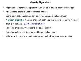
3. Greedy Algorithms Greedy algorithms typically consist of • A set of candidate solutions • Function that checks if the candidates are feasible • Selection function indicating at a given time which is the most promising candidate not yet used • Objective functiongiving the value of a solution; this is the function we are trying to optimize

4. Step by Step Approach • Initially, the set of chosen candidates is empty • At each step, add to this set the best remaining candidate; this is guided by selection function. • If increased set is no longer feasible, then remove the candidate just added; else it stays. • Each time the set of chosen candidates is increased, check whether the current set now constitutes a solution to the problem. When a greedy algorithm works correctly, the first solution found in this way is always optimal.

5. Examples of Greedy Algorithms • Graph Algorithms • Breath First Search (shortest path 4 un-weighted graph) • Dijkstra’s (shortest path) Algorithm • Minimum Spanning Trees • Data compression • Huffman coding • Scheduling • Activity Selection • Minimizing time in system • Deadline scheduling • Other Heuristics • Coloring a graph • Traveling Salesman • Set-covering

6. Elements of Greedy Strategy • Greedy-choice property: A global optimal solution can be arrived at by making locally optimal (greedy) choices • Optimal substructure: an optimal solution to the problem contains within it optimal solutions to sub-problems • Be able to demonstrate that if A is an optimal solutioncontainings1, then the setA’ = A - {s1} is an optimal solution to a smaller problem w/os1.

7. Analysis • The selection function is usually based on the objective function; they may be identical. But, often there are several plausible ones. • At every step, the procedure chooses the best candidate, without worrying about the future. It never changes its mind: once a candidate is included in the solution, it is there for good; once a candidate is excluded, it’s never considered again. • Greedy algorithms do NOT always yield optimal solutions, but for many problems they do.

8. Breadth-First Traversal • A breadth-first traversal • visits a vertex and • then each of the vertex's neighbors • before advancing Cost ? O(|V|+|E|)

9. 2 3 3 2 2 3 1 S S S 2 1 1 2 3 2 3 Finished Discovered Undiscovered Breadth-First Traversal Implementation?

10. Example (BFS) r s t u    0     v w y x Q: s 0

11. Example (BFS) r s t u   0 1    1 v w y x Q: w r 1 1

12. Example (BFS) r s t u 2  0 1  2  1 v w y x Q: r t x 1 2 2

13. Example (BFS) r s t u 2  0 1 2  2 1 v w y x Q: t x v 2 2 2

14. Example (BFS) r s t u 2 0 3 1 2  2 1 v w y x Q: x v u 2 2 3

15. Example (BFS) r s t u 2 0 3 1 2 3 2 1 v w y x Q: v u y 2 3 3

16. Example (BFS) r s t u 2 0 3 1 2 3 2 1 v w y x Q: u y 3 3

17. Example (BFS) r s t u 2 0 3 1 2 3 2 1 v w y x Q: y 3

18. Example (BFS) r s t u 2 0 3 1 2 3 2 1 v w y x Q:

19. Example (BFS) r s t u 2 0 3 1 2 3 2 1 v w y x Breath First Tree

20. r r s s t t u u 2 0 0 3 1 2 3 2 1 v v w w y y x x BFS : Application • Solves the shortest path problem for un-weighted graph

21. Dijkstra’s algorithm (4.4) 1 10 9 2 3 s 4 6 7 5 2 y x An adaptation of BFS

22. Example u v 1   10 9 2 3 0 s 4 6 7 5   2 y x

23. Example u v 1 10  10 9 2 3 0 s 4 6 7 5  5 5 2 y x

24. Example u v 1 8 14 10 9 2 3 0 s 4 6 7 5 7 7 5 2 y x

25. Example u v 1 8 8 13 10 9 2 3 0 s 4 6 7 5 7 5 2 y x

26. Example u v 1 9 8 9 10 9 2 3 0 s 4 6 7 5 7 5 2 y x

27. Example u v 1 8 9 10 9 2 3 0 s 4 6 7 5 7 5 2 y x

28. Dijkstra’s Algorithm • Assumes no negative-weight edges. • Maintains a set S of vertices whose shortest path from s has been determined. • Repeatedly selects u in V – S with minimum shortest path estimate (greedy choice). • Store V – S in priority queue Q. Cost: ? O(V2)

29. Dijkstra’s Algorithm

30. Minimal Spanning Trees Minimal Spanning Tree (MST) Problem: Input: An undirected, connected graph G. Output: The subgraph of G that • keeps the vertices connected; • has minimum total cost; (the sum of the values of the edges in the subset is at the minimum)

31. MST Example

32. Step by Step Greedy Approach • Initially, the set of chosen candidates is empty • At each step, add to this set the best remaining candidate; this is guided by selection function. • If increased set is no longer feasible, then remove the candidate just added; else it stays. • Each time the set of chosen candidates is increased, check whether the current set now constitutes a solution to the problem. When a greedy algorithm works correctly, the first solution found in this way is optimal.

33. MST Example

34. Greedy Algorithms • Kruskal's algorithm. Start with T = . Consider edges in ascending order of cost. Insert edge e in T unless doing so would create a cycle. • Prim's algorithm. Start with some root node s and greedily grow a tree T from s outward. At each step, add the cheapest edge e to T that has exactly one endpoint in T. • Reverse-Delete algorithm. Start with T = E. Consider edges in descending order of cost. Delete edge e from T unless doing so would disconnect T. • All three algorithms produce an MST.

35. Kruskal’s MST Algorithm • choose each vertex to be in its own MST; • merge two MST’s that have the shortest edge between them; • repeat step 2 until no tree to merge. • Implementation ? • Union-Find

36. Prim’s MST Algorithm A greedy algorithm. • choose any vertex N to be the MST; • grow the tree by picking the least cost edge connected to any vertices in the MST; • repeat step 2 until the MST includes all the vertices.

37. Prim’s MST demo http://www-b2.is.tokushimau.ac.jp/~ikeda/ suuri/dijkstra/PrimApp.shtml?demo1

38. (smallest polar angle w.r.t. p ) (smallest polar angle w.r.t. p ) (smallest polar angle w.r.t. p ) (smallest polar angle w.r.t. p ) (smallest polar angle w.r.t. p ) 1 5 4 0 2 p p p p p p p 3 2 4 6 0 5 1 (lowest point) Convex Hull - Jarvis’ March A “package wrapping” technique - Greedy

39. Jarvis’s March Greedy algorithm O(nh) time in total.

40. Huffman Coding Huffman codes –- very effective technique for compressing data, saving 20% - 90%.

41. Coding Problem: • Consider a data file of 100,000 characters • You can safely assume that there are many a,e,i,o,u, blanks, newlines, few q, x, z’s • Want to store it compactly Solution: • Fixed-length code, ex. ASCII, 8 bits per character • Variable length code, Huffman code (Can take advantage of relative freq of letters to save space)

42. 000 360 001 126 010 126 011 111 100 96 101 72 110 21 111 6 918 Example • Fixed-length code, need ? bits for each char 3 Char Frequency Code Total Bits E 120 L 42 D 42 U 37 C 32 M 24 K 7 Z 2

43. 37 E:120 L:42 D:42 U:37 C:32 M:24 K:7 Z:2 Example (cont.) Char Code 0 1 0 1 1 0 0 1 0 1 0 1 0 1  Complete binary tree

44. Example (cont.) • Variable length code (Can take advantage of relative freq of letters to save space) - Huffman codes Char Code

45. Huffman Tree Construction (1) • Associate each char with weight (= frequency) to form a subtree of one node (char, weight) • Group all subtrees to form a forest • Sort subtrees by ascending weight of subroots • Merge the first two subtrees (ones with lowest weights) • Assign weight of subroot with sum of weights of two children. • Repeat 3,4,5 until only one tree in the forest

46. Huffman Tree Construction (2)

47. M Huffman Tree Construction (3)

48. char Freq C 32 128 D 42 126 E 120 120 M 24 120 K 7 42 L 42 126 U 37 111 Z 2 12 785 Assigning Codes Compare with: 918 ~15% less Code Bits 1110 101 0 11111 111101 110 100 111100

49. Huffman Coding Tree

50. Coding and Decoding Char Code • DEED: • MUCK: 010000000010 101011100110 Char Code • DEED: • MUCK: 10100101 111111001110111101