Download
1 / 37
380 likes | 799 Views
ANALYSIS AND DESIGN OF ALGORITHMS. UNIT-V. CHAPTER 12:. COPING WITH THE LIMITATIONS OF ALGORITHM POWER. OUTLINE. Backtracking n-Queens Problem Hamiltonian Circuit Problem Subset-Sum Problem Branch-and-Bound Assignment Problem Knapsack Problem Traveling Salesman Problem. Backtracking.

E N D
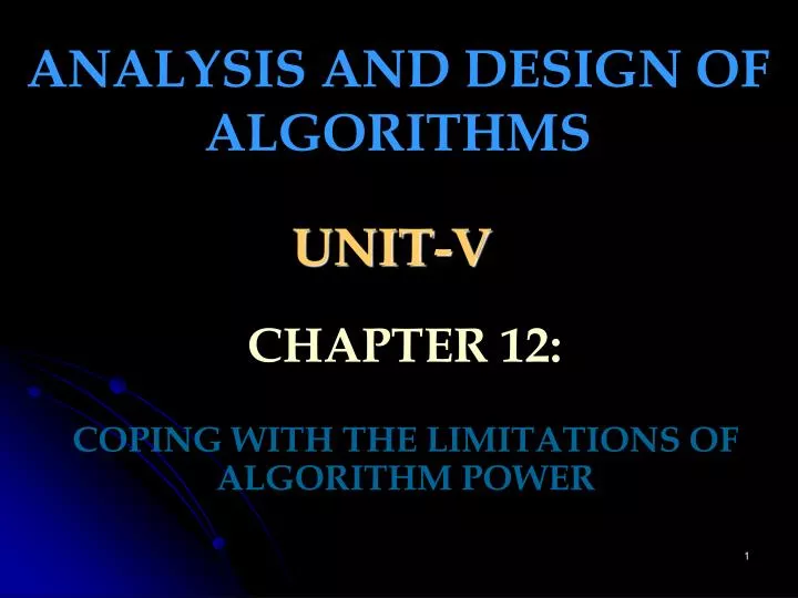
ANALYSIS AND DESIGN OF ALGORITHMS UNIT-V CHAPTER 12: COPING WITH THE LIMITATIONS OF ALGORITHM POWER
OUTLINE • Backtracking • n-Queens Problem • Hamiltonian Circuit Problem • Subset-Sum Problem • Branch-and-Bound • Assignment Problem • Knapsack Problem • Traveling Salesman Problem
Backtracking The principal idea is to construct solutions one component at a time and evaluate such partially constructed candidates as follows. If a partially constructed solution can be developed further without violating the problem’s constraints, it is done by taking the first remaining legitimate option for the next component. If there is no legitimate option for the next component, no alternatives for any remaining component need to be considered. In this case, the algorithm backtracks to replace the last component of the partially constructed solution with its next option.
Backtracking This kind of processing is often implemented by constructing a tree of choices being made, called the state-space tree. Itsroot represents an initial state before the search for a solution begins. The nodes of the first level in the tree represent the choices made for the first component of a solution, the nodes of the second level represent the choices for the second component, and so on. A node in a state-space tree is said to be promising if it corresponds to a partially constructed solution that may still lead to a complete solution; otherwise, it is callednonpromising.
Backtracking Leaves represent either nonpromising dead ends or complete solutions found by the algorithm. In the majority of cases, a state-space tree for a backtracking algorithm is constructed in the manner of depth-first search. If the current node turns out to be nonpromising, the algorithm backtracks to the node’s parent to consider the next possible option for its last component; if there is no such option, it backtracks one more level up the tree, and so on. Finally, if the algorithm reaches a complete solution to the problem, it either stops (if just one solution is required) or continues searching for other possible solutions.
Example: n-Queens Problem • The problem is to place n queens on an n-by-n chessboard so that no two queens attack each other by being in the same row or in the same column or on the same diagonal. Figure: Board for the four-queens problem.
N-Queens Problem For n=1, the problem has a trivial solution, and it is easy to see that there is no solution for n=2 and n=3. So let us consider the four-queens problem and solve it by the backtracking technique. We start with the empty board and then place queen 1 in the first possible position of its row, which is in column 1 of row 1. Then we place queen 2, after trying unsuccessfully columns 1 and 2, in the first acceptable position for it, which is square (2,3), the square in row 2 and column 3. This proves to be a dead end because there is no acceptable position for queen 3. So, the algorithm backtracks and puts queen 2 in the next possible position at (2,4). Then queen 3 is placed at (3, 2), which proves to be another dead end. The algorithm then backtracks all the way to queen1 and moves it to (1, 2). Queen2 then goes to (2, 4), queen3 to (3, 1), and queen4 to (4, 3) which is a solution to the problem.
Figure: State-space tree of solving the four-queens problem by backtracking. × denotes an unsuccessful attempt to place a queen in the indicated column. The numbers above the nodes indicate the order in which the nodes are generated.
Hamiltonian Circuit Problem we make vertex athe root of the state-space tree. The first component of our future solution, if it exists, is a first intermediate vertex of a Hamiltonian circuit to be constructed. Using the alphabet order to break the three-way tie among the vertices adjacent to a, we select vertex b. From b, the algorithm proceeds to c, then to d, then to e, and finally to f, which proves to be a dead end.
Hamiltonian Circuit Problem So the algorithm backtracks from f to e, then to d, and then to c, which provides the first alternative for the algorithm to pursue. Going from c to e eventually proves useless, and the algorithm has to backtrack from e to c and then to b. From there, it goes to the vertices f , e, c, and d, from which it can legitimately return to a, yielding the Hamiltonian circuit a, b, f , e, c, d, a. If we wanted to find another Hamiltonian circuit, we could continue this process by backtracking from the leaf of the solution found.
Figure: State-space tree for finding a Hamiltonian circuit. The numbers above the nodes of the tree indicate the order in which the nodes are generated.
Subset-Sum Problem • The subset-sum problem finds a subset of a given set S=(s1, . . . , sn} of n positive integers whose sum is equal to a given positive integer d. For example: for S={1, 2, 5, 6, 8} and d =9, there are two solutions: {1, 2, 6} and {1, 8}. • It is convenient to sort the set’s elements in increasing order. So we will assume that s1 ≤ s2 ≤ . . . ≤ sn. • The state-space tree can be constructed as a binary tree like that shown in next slide for the instance S={3, 5, 6, 7} and d=15. • The root of the tree represents the starting point, with no decisions about the given elements made as yet. • Its left and right children represent, respectively, inclusion and exclusion of s1 in a set being sought.
Subset-sum Problem 0 with 3 3 0 with 5 w/o 5 with 5 w/o 5 8 3 5 0 with 6 w/o 6 with 6 with 6 x w/o 6 w/o 6 14 0+13<15 8 9 3 11 5 x with 7 x x x x w/o 7 9+7>15 3+7<15 14+7>15 11+7>15 5+7<15 15 8 solution x 8<15 Figure: Complete state-space tree of the backtracking algorithm applied to the instance S={3, 5, 6, 7} and d=15 of the subset-sum problem. The number inside a node is the sum of the elements already included in subsets represented by the node. The inequality below a leaf indicates the reason for its termination.
Subset-Sum Problem • Similarly, going to the left from a node of the first level corresponds to inclusion of s2, while going to the right corresponds to its exclusion, and so on. • Thus, a path from the root to a node on the ith level of the tree indicates which of the first i numbers have been included in the subsets represented by that node. We record the value of s‘, the sum of these numbers, in the node. • If s‘ is equal to d, we have a solution to the problem. We can either report this result and stop or, if all the solutions need to be found, continue by backtracking to the node’s parent. • If s‘ is not equal to d, we can terminate the node as nonpromising if either of the following two inequalities holds: s‘ + si+1 > d (the sum s’ is too large) n s’ + ∑ sj < d (the sum s’ is too small). j=i+1
Backtracking: General Remark • An output of a backtracking algorithm can be thought of as an n-tuple (x1, x2, . . . , xn) where each coordinate xi is an element of some finite linearly ordered set Si. For example, for the n-queens problem, each Si is the set of integers (column numbers) 1 through n. • The tuple may need to satisfy some additional constraints (eg., the nonattacking requirements in the n-queens problem). • Depending on the problem, all solution tuples can be of the same length (the n-queens and the Hamiltonian circuit problem) or of different lengths (the subset-sum problem).
Backtracking: General Remark • A backtracking algorithm generates, explicitly or implicitly, a state- space tree; its nodes represents partially constructed tuples with the first i coordinates defined by the earlier actions of the algorithm. • If such a tuple (x1, x2, . . . , xi) is not a solution, the algorithm finds the next element in Si+1 that is consistent with the values of (x1, x2, . . . xi) and the problem’s constraints and adds it to the tuple as its (i+1) st coordinate. If such an element does not exist, the algorithm backtracks to consider the next value of xi, and so on.
Backtracking: General Remark To start a backtracking algorithm, the following pseudocode can be called for i=0; X[1. . . 0] represents the empty tuple.
Backtracking: General remark It is typically applied to difficult combinatorial problems for which no efficient algorithms for finding exact solutions possibly exist. Unlike the exhaustive search approach, which is doomed to be extremely slowfor all instances of a problem, backtracking at least holds a hope for solving some instances of nontrivial sizes in an acceptable amount of time. This is especially true for optimization problems. Even if backtracking does not eliminate any elements of a problem’s state space and ends up generating all its elements, it provides a specific technique for doing so, which can be of value in its own right.
Branch-and-Bound In the standard terminology of optimization problems, a feasible solutionis a point in the problem’s search space that satisfies all the problem’s constraints (eg., Hamiltonian circuit etc). An optimal solution is a feasible solution with the best value of the objective function (eg., the shortest Hamiltonian circuit etc).
Branch-and-Bound 3 Reasons for terminating a search path at the current node in a state-space tree of a branch-and-bound algorithm: The value of the node’s bound is not betterthan the value of the best solution seen so far. The node represents no feasible solutionsbecause the constraints of the problem are already violated. The subset of feasible solutions represented by the node consists of a singlepoint—in this case we compare the value of the objective function for this feasible solution with that of the best solution seen so far and update the latter with the former if the new solution is better.
Assignment Problem • Let us illustrate the branch-and-bound approach by applying it to the problem of assigning n people to n jobs so that the total cost of the assignment is as small as possible. • An instance of the assignment problem is specified by an n–by-n cost matrix C so that we can state the problem as follows: select one element in each row of the matrix so that no two selected elements are in the same column and their sum is the smallest possible. job 1 job 2 job 3 job4 9 2 7 8 person a 6 4 3 7 person b C = 5 8 1 8 person c 7 6 9 4 person d • It is clear that the cost of any solution, including an optimal one, cannot be smaller than the sum of the smallest elements in each of the matrix’s rows. For above instance, this sum is 2+3+1+4 = 10. It is just a lower bound on the cost of any legitimate selection.
Assignment Problem • We can and will apply the same thinking to partially constructed solutions. For example, for any legitimate selection that selects 9 from the first row, the lower bound will be 9 + 3 + 1 + 4 = 17. • Rather than generating a single child of the last promising node as we did in backtracking, we will generate all the children of the most promising node among nonterminated leaves in the current tree. • It is sensible to consider a node with the best bound as most promising, although this does not, of course, preclude the possibility that an optimal solution will ultimately belong to a different branch of the state-space tree. This variation of the strategy is called the best-first branch-and-bound. • We start with the root that corresponds to no elements selected from the cost matrix. The lower-bound value for the root, denoted lb, is 10. The nodes on the first level of the tree correspond to selections of an element in the first row of the matrix, i.e., a job for person a (refer next slide).
Branch-and-Bound: Assignment Problem 0 start lb = 2 + 3 + 1 + 4 = 10 1 2 3 4 a → 1 lb = 9 + 3 + 1 + 4 = 17 a → 2 lb = 2 + 3 + 1 + 4 = 10 a → 3 lb = 7 + 4 + 5 + 4 = 20 a → 4 lb = 8 + 3 + 1 + 6 = 18 Figure: Levels 0 and 1 of the state-space tree for the instance of the assignment problem being solved with the best-fit branch-and bound algorithm. The number above a node shows the order in which the node was generated. A node’s fields indicate the job number assigned to person a and the lower bound value, lb, for this node.
Assignment Problem • So we have four live leaves (node1 through 4) that may contain an optimal solution. The most promising of them is node 2 because it has the smallest lower-bound value. • Following our best-first search strategy, we branch out from that node first by considering the three different ways of selecting an element from the second row and not in the second column – the three different jobs that can be assigned to person b (refer next slide). • Of the six live leaves (nodes 1, 3, 4, 5, 6, and 7) that may contain an optimal solution, we again choose the one with the smallest lower bound, node 5. • First, we consider selecting the third column’s elements from c’s row (i.e., assigning person c to job 3); this leaves us with no choice but to select the element from the fourth column of d’s row (assigning person d to job 4).
Branch-and-Bound: Assignment Problem 0 start lb = 10 1 4 2 3 a → 1 lb = 17 a → 2 lb = 10 a → 3 lb = 20 a → 4 lb = 18 6 7 5 b → 1 lb = 13 b → 3 lb = 14 b → 4 lb = 17 Figure: Levels 0, 1, and 2 of the state-space tree for the instance of the assignment problem being solved with the best-first branch-and- bound algorithm.
Assignment Problem • This yields leaf 8 (refer next slide), which corresponds to the feasible solution {a → 2, b → 1, c → 3, d → 4} with the total cost of 13. • Its sibling, node 9, corresponds to the feasible solution {a → 2, b → 1, c → 4, d → 3} with the total cost of 25. Since its cost is larger than the cost of the solution represented by leaf 8, node 9 is simply terminated. • Now, as we inspect each of the live leaves of the last state-space tree (nodes 1, 3, 4, 6, and 7 in next slide), we discover that their lower-bound values are not smaller than 13, the value of the best selection seen so far (leaf 8). Hence, we terminate all of them and recognize the solution represented by leaf 8 as the optimal solution to the problem.
Branch-and-Bound: Assignment Problem 0 start lb = 10 4 1 2 3 a → 1 lb = 17 a → 2 lb = 10 a → 3 lb = 20 a → 4 lb = 18 x x x 5 6 7 b → 1 lb = 13 b → 3 lb = 14 b → 4 lb = 17 x x 8 9 c → 4 d → 3 c → 3 d → 4 cost = 25 cost = 13 inferior solution solution Figure: Complete state-space tree for the instance of the assignment problem solved with the best-first branch-and-bound algorithm.
Knapsack Problem • It is convenient to order the items of a given instance in decreasing order by their value-to-weight ratios. • Then the first item gives the best payoff per weight unit and the last one gives the worst payoff per weight unit: v1/w1 ≥ v2/w2 ≥ . . . ≥ vn/wn. • The state-space tree for this problem is shown in next slide. • Each node on the ith level of this tree, 0 ≤ i ≤ n, represents all the subsets of n items that include a particular selection made from the first i ordered items. • This particular selection is uniquely determined by the path from the root to the node: a branch going to the left indicates the inclusion of the next item, while a branch going to the right indicates its exclusion.
Knapsack Problem • We record the total weight w and the total value v of this selection in the node, along with some upper bound ub on the value of any subset that can be obtained by adding zero or more items to this selection. • A simple way to compute the upper bound ub is to add to v, the total value of the items already selected, the product of the remaining capacity of the knapsack W-w and the best per unit payoff among the remaining items, which is vi+1/wi+1: ub = v + (W – w)(vi+1/wi+1). • Let us apply the branch-and-bound algorithm to the following instance of the knapsack problem( Items are reordered in descending order of their value-to-weight ratios). item weight value value/weight 1 4 $40 10 2 7 $42 6 3 5 $25 5 Capacity W=10 4 3 $12 4
Branch-and-Bound: Knapsack Problem 0 w = 0, v = 0 ub = 100 with 1 w/o 1 1 2 w = 0, v = 0 ub = 60 w = 4, v = 40 ub = 76 with 2 w/o 2 x 4 3 inferior to node 8 w = 11 w = 4, v = 40 ub = 70 x with 3 w/o 3 5 6 not feasible w = 9, v = 65 ub = 69 w = 4, v = 40 ub = 64 with 4 x w/o 4 7 8 w = 12 w = 9, v = 65 ub = 65 inferior to node 8 Figure: State-space tree of the branch-and-bound algorithm for the instance of the knapsack problem. x not feasible optimal solution
Knapsack Problem • At the root of the state-space tree, no items have been selected as yet. Hence, both the total weight of the items already selected w and their total value v are equal to 0. The value of the upper bound computed is $100. • Node1, the left child of the root, represents the subsets that include item1. The total weight and value of the items already included are 4 and $40, respectively; the value of the upper bound is 40 + (10 - 4) * 6 = $76. • Node2 represents the subsets that do not include item1. Accordingly, w = 0, v = $0, and ub = 0 + (10 – 0) * 6 = $60. • Since node1 has a larger upper bound than the upper bound of node2, it is more promising for this maximization problem, and we branch from node1 first.
Knapsack Problem • Node 1’s children –node 3 and node 4 – represent subsets with item1 and with and without item2, respectively. Since the total weight of every subset represented by node 3 exceeds the knapsack’s capacity, node 3 can be terminated immediately. • Node 4 has the same values of w and v as its parent; the upper bound ub is equal to 40 + (10 – 4) * 5 = $70. • Selecting node 4 over node 2 for the next branching, we get nodes 5 and 6 by respectively including and excluding item3. • Branching from node 5 yields node 7, which represents no feasible solutions, and node 8, which represents just a single subset {1, 3}. • The remaining live nodes 2 and 6 have smaller upper-bound values than the value of the solution represented by node 8. Hence, both can be terminated making subset {1, 3} of node 8 the optimal solution to the problem.
Traveling Salesman Problem • We can compute a lower bound on the length l of any tour as follows: • For each city i, 1 ≤ i ≤ n, find the sum si of the distances from city i to the two nearest cities; • compute the sum s of these n numbers; • divide the result by 2; and, if all the distances are integers, round up the result to the nearest integer: lb = s/2 . For example, for the instance in below figure, the above formula yields lb = [(1+3) + (3+6) + (1+2) + (3+4) + (2+3)]/2 = 14. 3 a b 6 5 7 1 9 8 4 c d 2 3 Figure: Weighted graph. e
Traveling Salesman Problem • For any subset of tours that must include particular edges of a given graph, we can modify lower bound accordingly. • For example, for all the Hamiltonian circuits of the graph in below figure that must include edge (a, d), we get the following lower bound by summing the lengths of the two shortest edges incident with each of the vertices, with the required inclusion of edges (a, d) and (d, a) : [(1+5) + (3+6) + (1+2) + (3+5) + (2+3)]/2 = 16. 3 a b 6 5 7 1 9 8 4 c d 2 3 Figure: Weighted graph. e
Traveling Salesman Problem • We now apply the branch-and bound algorithm, with the bounding function given by formula lb = s/2 , to find the shortest Hamiltonian circuit for the graph shown below. • We can consider only tours that start at a. Since the graph is undirected, we can generate only tours in which b is visited before c. • In addition, after visiting n-1 = 4 cities, a tour has no choice but to visit the remaining unvisited city and return to the starting one. • The state-space tree tracing the algorithm’s application is given in next slide. 3 a b 6 5 7 1 9 8 4 c d 2 3 Figure: Weighted graph. e
Branch-and-Bound: Traveling Salesman Problem 0 a lb = 14 4 1 2 3 a , b lb = 14 a , c a , d lb = 16 a , e lb = 19 x x x lb >= l of node 11 b is not before c lb > l of node 11 5 6 7 a, b, d lb = 16 a, b, c lb = 16 a, b, e lb = 19 x 8 10 lb > l of node 11 9 11 a, b, c, d, (e, a) a, b, d, c, (e, a) a, b, d, e, (c, a) a, b, c, e, (d, a) l = 24 l = 19 l = 24 l = 16 First tour inferior tour optimal tour better tour Figure: State-space tree of the branch-and-Bound algorithm to find the shortest Hamiltonian circuit in this graph. The list of vertices in a node specifies a beginning part of the Hamiltonian circuits represented by the node.