Download
1 / 18
190 likes | 319 Views
Maximin D-optimal designs for binary longitudinal responses. Fetene B. Tekle, Frans E. S. Tan and Martijn P. F. Berger Department of Methodology and Statistics, Maastricht University, Maastricht, NL. DEMA2008 11 August to 15 August 2008

E N D
Maximin D-optimal designs for binary longitudinal responses Fetene B. Tekle, Frans E. S. Tan and Martijn P. F. Berger Department of Methodology and Statistics, Maastricht University, Maastricht, NL DEMA2008 11 August to 15 August 2008 Isaac Newton Institute for Mathematical Sciences, Cambridge, UK
2 Outline • Introduction • Objectives • Model and variance-covariances • D-optimality • Relative efficiency • Maximin D-optimal designs • Numerical study and results • Concluding remarks
3 • Introduction Problem The optimality criteria for non linear models depend on unknown parameter values (Silvey, 1980; Atkinson and Donev, 1996), designing experiments requires full knowledge of the regression coefficients. Solutions: locally optimal (Fedorov and Müller, 1997)
4 • Introduction (contd.) Solutions: • Sequential procedure (Wu, 1985; Sitter and Forbes, 1997; and Sitter and Wu, 1999), • Bayesian procedure (Chaloner, 1989; Chaloner and Larntz, 1989; Atkinson et al., 1993; Chaloner and Verdinelli, 1995; Dette, 1996 and Han and Chaloner, 2004), and • Maximin approach (Müller, 1995; Dette, 1997; Müller and Pazman, 1998; Dette and Sahm, 1997, 1998; King and Wong, 2000; Imhof, 2001; Ouwens et al., 2002, 2006; Braess and Dette, 2007).
5 • Objectives • Binary longitudinal responses (Mixed-effects logistic model) • Investigate locally D-optimal designs • Maximin approach with D-optimality • Identify maximin D-optimal designs, • Identify the optimum number of repeated measurements needed for a longitudinal study with binary responses.
Model and variance-covariances 6 The model (1)
Model and variance-covariances …… 7 Estimation and variances (2) a) PQL method: An approximate variance-covariance matrix for the parameters estimator is (Breslow and Clayton, 1993): (3) where V is the block-diagonal matrix with blocks q x q matrices given by: (4) where wi is a diagonal matrix of the conditional variances of the responses given the random effects, the q x r matrix z is made by having as rows.
Model and variance-covariances …… 8 b) Extended GEE method with serial correlations (Zeger et al., 1998; Molenberghs and Verbeke, 2005): (5) where the working variance-covariance of the responses vi is given by: (6) The q x q matrixR(ρ) is the correlation matrix of the responses over time (AR(1) structure is assumed).
D-optimality 9 A design is D-optimal if (Atkinson and Donev, 1996) where the design space of q x 1 time vectors be denoted by (7)
Relative Efficiency (RE) 10 RE is used to compare two designs (8)
Maximin D-optimal designs 11 A design is maximin D-optimal for , if it maximizes the smallest relative efficiency over The maximin D-optimal design maximizes the minimum relative efficiency among all designs with q time points and the corresponding maximin efficiency is given by: (9)
Numerical study and Results 12 • Locally D-optimal and maximin D-optimal designs within the time interval [-1, 1]. • Random intercept, and random intercept and slope models with • linear, • quadratic and • cubic terms of time. • Two sets of intervals of parameters (0.0, 1.5) and (0.0, 3.0] for the maximin D-optimal designs. • A MATLAB code with fmincon function
14 • Optimal time points include the two end points of the study period (time interval) if a value of a regression parameter is small. • As q increases, the optimal locations of the additional time points are close to the optimal allocations of a design with q = p for the PQL method. • When serial correlation is introduced, the optimal locations of the additional time points move further to the center and the design resembles an equi-distance design.
17 Maximin designs that include the end points of the time interval with regression parameter values in (0.0, 1.5).
Concluding remarks 18 • Optimal design points may not include the two end points of the study period (time interval), • MMEs are large, • A maximin D-optimal design with number of repeated measurements q is equal to the number of regression parameters p is the most efficient design compared to designs with more number of repeated measurements. • Future work: ? Control for additional experimental variable(s) ? Dropouts