Download
1 / 21
210 likes | 394 Views
Workshop 1 Alternative models for clustered survival data. Log-linear model representation in parametric survival models. In most packages (SAS, R) survival models (and their estimates) are parametrized as log linear models

E N D
Log-linear model representationin parametric survival models • In most packages (SAS, R) survival models (and their estimates) are parametrized as log linear models • If the error term eij has extreme value distribution, then this model corresponds to • PH Weibull model with • AFT Weibull model with
The first data setbivariate survival data • Time to reconstitution of blood-milk barrier after mastitis • Two quarters are infected with E. coli • One quarter treated locally, other quarter not • Blood milk-barrier destroyed • Milk Na+ increases • Time to normal Na+ level
Reading in the data library(survival) bloodmilk<-read.table("c://bivariate.dat",header=T) cows<-bloodmilk$cows y<-bloodmilk$y uncens<-bloodmilk$uncens trt<-bloodmilk$trt heifer<-bloodmilk$heifer table(trt,uncens) uncens trt 0 1 0 28 72 1 19 81
Types of models fitted • Treatment effect • Parametric models with constant hazard • Unadjusted model • Marginal model • Fixed effects model • Parametric models based on Weibull distribution • Unadjusted model and coefficient interpretation • Models with unspecified baseline hazard • Stratified model • Semiparametric marginal model • Heifer effect • Fixed effects model with constant hazard • Stratified model
Exponential unadjusted model res.unadjust<-survreg(Surv(y,uncens)~trt,dist="exponential",data=bloodmilk) summary(res.unadjust) b.unadjust<- -res.unadjust$coef[2] v.unadjust<- sqrt(res.unadjust$var[2,2]) l.unadjust<-exp(-res.unadjust$coef[1]) Call: survreg(formula = Surv(y, uncens) ~ trt, data = bloodmilk, dist = "exponential") Value Std. Error z p (Intercept) 1.531 0.118 12.99 1.33e-38 trt -0.176 0.162 -1.09 2.77e-01 > l.unadjust (Intercept) 0.2162472
Exponential marginal model ncows<-length(levels(as.factor(cows))) bdel<-rep(NA,ncows) for (i in 1:ncows){ temp<-bloodmilk[bloodmilk$cows!=i,] bdel[i]<-survreg(Surv(y,uncens)~trt,data=temp,dist="exponential")$coeff[2]} sqrt(sum((bdel-b.unadjust)^2)) 0.1535
Exponential fixed effects model res.fixed<- survreg(Surv(y,uncens)~trt+as.factor(cows),dist="exponential",data=bloodmilk) summary(res.fixed) b.fix<- -res.fixed$coef[2] v.fix<- sqrt(res.fixed$var[2,2]) Call:survreg(formula = Surv(y, uncens) ~ trt + as.factor(cows), data = bloodmilk, dist = "exponential") Value Std. Error z p (Intercept) 2.10e+01 3331.692 0.00629 0.995 trt -1.85e-01 0.190 -0.96993 0.332 as.factor(cows)2 -1.88e+01 3331.692 -0.00564 0.995 … as.factor(cows)100 -1.86e+01 3331.692 -0.00557 0.996
Weibull unadjusted model (1) res.unadjustw<-survreg(Surv(y,uncens)~trt,dist="weibull",data=bloodmilk) summary(res.unadjustw) b.unadjustw<- -res.unadjustw$coef[2]/res.unadjustw$scale v.unadjustw<- sqrt(res.unadjustw$var[2,2]) l.unadjustw<-exp(-res.unadjustw$coef[1]/res.unadjustw$scale) r.unadjustw<-1/res.unadjustw$scale Call:survreg(formula = Surv(y, uncens) ~ trt, data = bloodmilk, dist = "weibull") Value Std. Error z p (Intercept) 1.533 0.1222 12.542 4.38e-36 trt -0.180 0.1681 -1.072 2.84e-01 Log(scale) 0.036 0.0695 0.518 6.04e-01 Scale= 1.04 b.unadjustw trt 0.17387 v.unadjustw 0.1681 l.unadjustw (Intercept) 0.2278757 r.unadjustw 0.9646458
Weibull unadjusted model (2) likelihood.unadjust.weib.exptransf<-function(p){ cumhaz<-exp(trt*p[2])*y^(exp(p[3]))*exp(p[1]) lnhaz<-uncens*(trt*p[2]+log(exp(p[1]))+log(exp(p[3]))+(exp(p[3])-1)*log(y) ) lik<- sum(cumhaz)-sum(lnhaz)} initial<-c(log(0.23),0.2,log(1)) res<-nlm(likelihood.unadjust.weib.exptransf,initial) l.unadjustw2<-exp(res$estimate[1]) b.unadjustw2<-res$estimate[2] r.unadjustw2<-exp(res$estimate[3]) 0.228 0.174 0.965
Weibull unadjusted model (3) likelihood.unadjust.weib<-function(p){ cumhaz<-exp(trt*p[2])*y^(p[3])*p[1] lnhaz<-uncens*(trt*p[2]+log(p[1])+log(p[3])+(p[3]-1)*log(y)) lik<- sum(cumhaz)-sum(lnhaz)} initial<-c(exp(res$estimate[1]),res$estimate[2],exp(res$estimate[3])) res.unadjustw2<-nlm(likelihood.unadjust.weib,initial,iterlim=1,hessian=T) l.unadjustw2<-res.unadjustw2$estimate[1] b.unadjustw2<-res.unadjustw2$estimate[2] r.unadjustw2<-res.unadjustw2$estimate[3] v.unadjustw2<-sqrt(solve(res.unadjustw2$hessian)[2,2]) 0.228 0.174 0.965 0.162
Stratified model res.strat<-coxph(Surv(y,uncens)~trt+strata(cows)) summary(res.strat) b.strat<-res.strat$coef[1] v.strat<-res.strat$coef[3] Call: coxph(formula = Surv(y, uncens) ~ trt + strata(cows)) n= 200 coef exp(coef) se(coef) z p exp(-coef) lower .95 upper .95 trt 0.131 1.14 0.209 0.625 0.53 0.878 0.757 1.72
Semiparametric marginal model (1) res.semimarg<-coxph(Surv(y,uncens)~trt+cluster(cows)) summary(res.semimarg) b.semimarg<-summary(res.semimarg)$coef[1] v.semimarg<-summary(res.semimarg)$coef[4] Call: coxph(formula = Surv(y, uncens) ~ trt + cluster(cows)) n= 200 coef exp(coef) se(coef) robust se z p lower .95 upper .95 trt 0.161 1.17 0.162 0.145 1.11 0.27 0.883 1.56 Rsquare= 0.005 (max possible= 0.999 ) Likelihood ratio test= 0.98 on 1 df, p=0.322 Wald test = 1.22 on 1 df, p=0.269 Score (logrank) test = 0.98 on 1 df, p=0.322, Robust = 1.23 p=0.268
Semiparametric marginal model (2) b.unadjust<-coxph(Surv(y,uncens)~trt)$coeff[1] ncows<-length(levels(as.factor(cows))) bdel<-rep(NA,ncows) for (i in 1:ncows){ temp<-bloodmilk[bloodmilk$cows!=i,] bdel[i]<- -coxph(Surv(y,uncens)~trt,data=temp)$coeff[1] } sqrt(sum((-bdel-b.unadjust)^2)) [1] 0.1468473
Fixed effects model with heifer,heifer first summary(survreg(Surv(y,uncens)~heifer+as.factor(cows),dist="exponential", data=bloodmilk)) Call:survreg(formula = Surv(y, uncens) ~ heifer + as.factor(cows),data=bloodmilk, dist = "exponential") Value Std. Error z p (Intercept) 2.09e+01 4723 4.42e-03 0.996 heifer -2.01e+01 6680 -3.01e-03 0.998 as.factor(cows)2 1.21e+00 4723 2.56e-04 1.000 ... as.factor(cows)100 -1.85e+01 4723 -3.92e-03 0.997
Fixed effects model with heifer,cow first summary(survreg(Surv(y,uncens)~as.factor(cows)+heifer,dist="exponential", data=bloodmilk)) Call:survreg(formula = Surv(y, uncens) ~ as.factor(cows) + as.factor(heifer),data=bloodmilk,dist="exponential") Value Std. Error z p (Intercept) 2.09e+01 4723 0.00442 0.996 as.factor(cows)2 -1.89e+01 4723 -0.00399 0.997 as.factor(cows)100 -1.85e+01 4723 -0.00392 0.997 as.factor(heifer)1 0.00e+00 6680 0.00000 1.000
Stratified model with heifer > summary(coxph(Surv(y,uncens)~heifer+strata(cows),data=bloodmilk)) Call:coxph(formula = Surv(y, uncens) ~ heifer + strata(cows), data = bloodmilk) n= 200 coef exp(coef) se(coef) z p exp(-coef) lower .95 upper .95 heifer NA NA 0 NA NA NA NA NA Rsquare= 0 (max possible= 0.471 ) Likelihood ratio test= 0 on 0 df, p=NaN Wald test = NA on 0 df, p=NA Score (logrank) test = 0 on 0 df, p=NaN Warning messages: 1: X matrix deemed to be singular; variable 1 in: coxph(Surv(y, uncens) ~ heifer + strata(cows), data = bloodmilk) 2: NaNs produced in: pchisq(q, df, lower.tail, log.p) 3: NaNs produced in: pchisq(q, df, lower.tail, log.p)
The data set: Time to first insemination • Database of regional Dairy Herd Improvement Association (DHIA) • Milk recording service • Artificial insemination • Select sample • Subset of 2567 cows from 49 dairy farms
Effect of initial ureum concentration • Fit the following models • Parametric models with constant hazard • Unadjusted model • Fixed effects model • Marginal model • Models with unspecified baseline hazard • Stratified model • Semiparametric marginal model • Fixed effects model


![[Alternative Ownership Models]](https://cdn2.slideserve.com/5345939/alternative-ownership-models-dt.jpg)