Download
1 / 30
310 likes | 368 Views
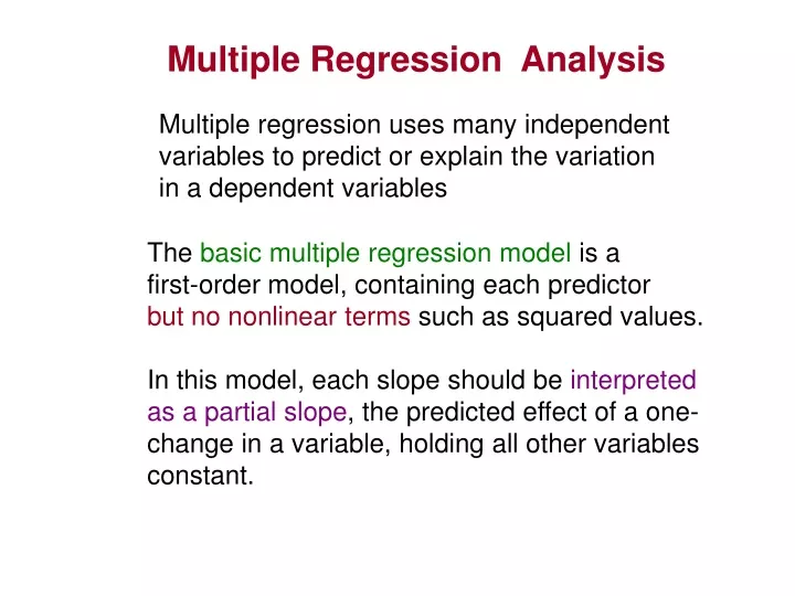
Multiple Regression Analysis. Multiple regression uses many independent variables to predict or explain the variation in a dependent variables. The basic multiple regression model is a first-order model, containing each predictor but no nonlinear terms such as squared values.

E N D
Multiple Regression Analysis Multiple regression uses many independent variables to predict or explain the variation in a dependent variables The basic multiple regression model is a first-order model, containing each predictor butno nonlinear terms such as squared values. In this model, each slope should be interpreted as a partial slope, the predicted effect of a one- change in a variable, holding all other variables constant.
Multiple Regression Analysis Estimating Equation Describing Relationship among Three Variables Estimating Equation Describing Relationship among n Variables
Multiple Regression Analysis – Example File: PPT_MultRegr The department is interested to know whether the amount of field audits and computer hours spent on tracking have yielded any results. Further the department has introduced the reward system for tracking the culprits. The data on actual unpaid taxes for ten cases is considered for analysis. Initially the regression of Actual Unpaid Taxes(Y) on Field Audits(X1) and Computer Hours(X2) was carried out and as a next step the Reward to Informants(X3) was also considered as a variable and analyzed. The analysis yielded the following SPSS outputs.
Multiple Regression and Correlation Analysis – Excel Output for 3 Independent Variables
Multiple Regression and Correlation Analysis – SPSS Output for 3 Independent Variables
Multiple Regression and Correlation Analysis Using two independent variables : Using three independent variables:
Coefficient of Determination • From the output, R2 = 0.983 • 98.3% of the variation in actual unpaid taxes is explained by the three independent variables. 1.7% remains unexplained.
Multiple Regression and Correlation Analysis Making inferences about Population Parameters 1. Inferences about an individual slope or whether a variable is significant 2. Regression as a whole
Multiple Regression and Correlation Analysis Inferences about the Regression as a Whole
Multiple Regression and Correlation Analysis Test Statistic Value of the test statistic:
Multiple Regression and Correlation Analysis Test of whether a variable is significant. Test whether reward to informants is a significant explanatory variable.
Multiple Regression and Correlation Analysis Test statistic, with n-2 degrees of freedom: Rejection Region
Multiple Regression and Correlation Analysis Value of the test statistic: Conclusion: The standardized regression coefficient is 9.6429 which is outside the acceptance region. Therefore we will reject the null hypothesis. The reward to informants is a significant explanatory variable.
Interpreting the Coefficients • b0 = - 45.796. This is the intercept, the value of y when all the variables take the value zero. Since the data range of all the independent variables do not cover the value zero, do not interpret the intercept. • b1 = 0.597. In this model, for each additional field audit, the actual unpaid taxes increases on average by .597% (assuming the other variables are held constant).
Estimating the Coefficients and Assessing the Model, Another Example • Where to locate a new motor inn? • La Quinta Motor Inns is planning an expansion. • Management wishes to predict which sites are likely to be profitable. • Several areas where predictors of profitability can be identified are: • Competition • Market awareness • Demand generators • Demographics • Physical quality
Physical Estimating the Coefficients and Assessing the Model, Example Operating Margin Profitability Market awareness Competition Customers Community Rooms Nearest Office space College enrollment Income Disttwn Median household income. Number of hotels/motels rooms within 3 miles from the site. Distance to the nearest La Quinta inn. Distance to downtown.
Estimating the Coefficients and Assessing the Model, Example • Data were collected from randomly selected 100 inns that belong to La Quinta, and ran for the following suggested model (Multiple Regr_Margin.sav): Margin = b0 + b1Rooms + b2Nearest + b3Office + b4College + b5Income + b6Disttwn
Regression Analysis, SPSS Output This is the sample regression equation (sometimes called the prediction equation) Margin = 38.139 - 0.008Number +1.646Nearest+ 0.020Office Space +0.212Enrollment + 0.413Income - 0.225Distance
Coefficient of Determination • From the printout, R2 = 0.525 • 52.5% of the variation in operating margin is explained by the six independent variables. 47.5% remains unexplained.
Testing the Validity of the Model • We pose the question: Is there at least one independent variable linearly related to the dependent variable? • To answer the question we test the hypothesis H0: B0 = B1 = B2 = … = Bk H1: At least one Bi is not equal to zero. • If at least one Bi is not equal to zero, the model has some validity.
Testing the Validity of the La Quinta Inns Regression Model • The hypotheses are tested by an ANOVA procedure ( the SPSS output) MSR/MSE k = n–k–1 = n-1 = SSR MSR=SSR/k MSE=SSE/(n-k-1) SSE
Testing the Validity of the La Quinta Inns Regression Model Conclusion: There is sufficient evidence to reject the null hypothesis in favor of the alternative hypothesis. At least one of the bi is not equal to zero. Thus, at least one independent variable is linearly related to y. This linear regression model is valid Fa,k,n-k-1 = F0.05,6,100-6-1=2.17 F = 17.14 > 2.17 Also, the p-value (Significance F) = 0.0000 Reject the null hypothesis.
Interpreting the Coefficients • b0 = 38.139. This is the intercept, the value of y when all the variables take the value zero. Since the data range of all the independent variables do not cover the value zero, do not interpret the intercept. • b1 = – 0.008. In this model, for each additional room within 3 mile of the La Quinta inn, the operating margin decreases on average by .008% (assuming the other variables are held constant).
Interpreting the Coefficients • b2 = 1.646. In this model, for each additional mile that the nearest competitor is to a La Quinta inn, the operating margin increases on average by 1.646% when the other variables are held constant. • b3 = 0.020.For each additional 1000 sq-ft of office space, the operating margin will increase on average by .02% when the othervariables are held constant. • b4 = 0.212. For each additional thousand students the operating margin increases on average by .212% when the othervariables are held constant.
Interpreting the Coefficients • b5 = 0.413. For additional $1000 increase in median household income, the operating margin increases on average by .413%, when the other variables remain constant. • b6 = -0.225. For each additional mile to the downtown center, the operating margin decreases on average by .225% when the other variables are held constant.
Test statistic Testing the Coefficients • The hypothesis for each bi is • SPSS printout H0: bi= 0 H1: bi¹ 0 d.f. = n - k -1
La Quinta Inns, Predictions • Predict the average operating margin of an inn at a site with the following characteristics: • 3815 rooms within 3 miles, • Closet competitor .9 miles away, • 476,000 sq-ft of office space, • 24,500 college students, • $35,000 median household income, • 11.2 miles distance to downtown center. MARGIN = 38.14 - 0.008(3815)+1.65(.9) + 0.020(476) +0.212(24.5) + 0.413(35) - 0.225(11.2) = 37.1%