Download
1 / 56
560 likes | 572 Views
Probability: The Study of Randomness 4.1 Randomness 4.2 Probability Models. Dal-AC FALL 2019. Objectives. 4.1 Randomness 4.2 Probability models Probability and Randomness Sample spaces Probability rules Assigning probabilities: finite number of outcomes

E N D
Probability: The Study of Randomness4.1 Randomness 4.2 Probability Models Dal-AC FALL 2019
Objectives 4.1 Randomness 4.2 Probability models • Probability and Randomness • Sample spaces • Probability rules • Assigning probabilities: finite number of outcomes • Assigning probabilities: equally likely outcomes • Independence and multiplication rule
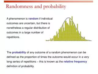
Randomness and probability A phenomenon is random if individual outcomes are uncertain, but there is nonetheless a regular distribution of outcomes in a large number of repetitions. The probability of any outcome of a random phenomenon can be defined as the proportion of times the outcome would occur in a very long series of repetitions.
The result of any single coin toss is random. But the result over many tosses is predictable, as long as the trials are independent (i.e., the outcome of a new coin flip is not influenced by the result of the previous flip). Coin toss The probability of heads is 0.5 = the proportion of times you get heads in many repeated trials. First series of tosses Second series
Two events are independent if the probability that one event occurs on any given trial of an experiment is not affected or changed by the occurrence of the other event. When are trials not independent? Imagine that these coins were spread out so that half were heads up and half were tails up. Close your eyes and pick one. The probability of it being heads is 0.5. However, if you don’t put it back in the pile, the probability of picking up another coin that is heads up is now less than 0.5. The trials are independent only when you put the coin back each time. It is called sampling with replacement.
Probability models Probability models describe, mathematically, the outcome of random processes. They consist of two parts: 1) S = Sample Space: This is a set, or list, of all possible outcomes of a random process. An event is a subset of the sample space. 2) A probability for each possible event in the sample space S. Example: Probability Model for a Coin Toss: S = {Head, Tail} Probability of heads = 0.5 Probability of tails = 0.5
H - HHH H M - HHM H S = { HHH, HHM, HMH, HMM, MHH, MHM, MMH, MMM } Note: 8 elements, 23 H - HMH M M - HMM M … … Sample spacesIt’s the question that determines the sample space. A. A basketball player shoots three free throws. What are the possible sequences of hits (H) and misses (M)? B. A basketball player shoots three free throws. What is the number of baskets made? S = { 0, 1, 2, 3 } C. A nutrition researcher feeds a new diet to a young male white rat. What are the possible outcomes of weight gain (in grams)? S = [0, ∞[ = (all numbers ≥ 0)
Coin Toss Example: S = {Head, Tail} Probability of heads = 0.5 Probability of tails = 0.5 Probability rules 1) Probabilities range from 0 (no chance of the event) to1 (the event has to happen). For any event A, 0 ≤ P(A) ≤ 1 Probability of getting a Head = 0.5 We write this as: P(Head) = 0.5 P(neither Head nor Tail) = 0 P(getting either a Head or a Tail) = 1 2) Because some outcome must occur on every trial, the sum of the probabilities for all possible outcomes (the sample space) must be exactly 1. P(sample space) = 1 Coin toss: S = {Head, Tail} P(head) + P(tail) = 0.5 + 0.5 =1 P(sample space) = 1
Venn diagrams: A and B disjoint Probability rules (cont’d ) 3) Two events A and B are disjoint if they have no outcomes in common and can never happen together. The probability that A or B occurs is then the sum of their individual probabilities. P(A or B) = “P(A U B)” = P(A) + P(B) This is the addition rule for disjoint events. A and B not disjoint Example:If you flip two coins, and the first flip does not affect the second flip: S = {HH, HT, TH, TT}. The probability of each of these events is 1/4, or 0.25. The probability that you obtain “only heads or only tails” is:P(HH or TT) = P(HH) + P(TT) = 0.25 + 0.25 = 0.50
Coin Toss Example: S ={Head, Tail} Probability of heads = 0.5 Probability of tails = 0.5 Probability rules (cont’d) 4) The complement of any event A is the event that A does not occur, written as Ac. The complement rule states that the probability of an event not occurring is 1 minus the probability that is does occur. P(not A) = P(Ac) = 1 −P(A) Tailc = not Tail = Head P(Tailc) = 1 −P(Head) = 0.5 Venn diagram: Sample space made up of an event A and its complementary Ac, i.e., everything that is not A.
Probabilities: finite number of outcomes Finite sample spaces deal with discrete data—data that can only take on a limited number of values. These values are often integers or whole numbers. The individual outcomes of a random phenomenon are always disjoint. The probability of any event is the sum of the probabilities of the outcomes making up the event (addition rule). Throwing a die: S = {1, 2, 3, 4, 5, 6}
M&M candies If you draw an M&M candy at random from a bag, the candy will have one of six colors. The probability of drawing each color depends on the proportions manufactured, as described here: What is the probability that an M&M chosen at random is blue? S = {brown, red, yellow, green, orange, blue} P(S) = P(brown) + P(red) + P(yellow) + P(green) + P(orange) + P(blue) = 1 P(blue) = 1 – [P(brown) + P(red) + P(yellow) + P(green) + P(orange)] = 1 – [0.3 + 0.2 + 0.2 + 0.1 + 0.1] = 0.1 What is the probability that a random M&M is either red, yellow, or orange? P(red or yellow or orange) = P(red) + P(yellow) + P(orange) = 0.2 + 0.2 + 0.1 = 0.5
Probabilities: equally likely outcomes We can assign probabilities either: • empirically from our knowledge of numerous similar past events • Mendel discovered the probabilities of inheritance of a given trait from experiments on peas without knowing about genes or DNA. • or theoretically from our understanding of the phenomenon and symmetries in the problem • A 6-sided fair die: each side has the same chance of turning up • Genetic laws of inheritance based on meiosis process If a random phenomenon has k equally likely possible outcomes, then each individual outcome has probability 1/k. And, for any event A:
Dice You toss two dice. What is the probability of the outcomes summing to 5? This isS: {(1,1), (1,2), (1,3), ……etc.} There are 36 possible outcomes in S, all equally likely (given fair dice). Thus, the probability of any one of them is 1/36. P(the roll of two dice sums to 5) = P(1,4) + P(2,3) + P(3,2) + P(4,1) = 4 / 36 = 0.111
The gambling industry relies on probability distributions to calculate the odds of winning. The rewards are then fixed precisely so that, on average, players lose and the house wins. The industry is very tough on so called “cheaters” because their probability to win exceeds that of the house. Remember that it is a business, and therefore it has to be profitable.
Coin Toss Example: S = {Head, Tail} Probability of heads = 0.5 Probability of tails = 0.5 Probability rules (cont’d) 5) Two events A and B are independent if knowing that one occurs does not change the probability that the other occurs. If A and B are independent, P(A and B) = P(A)P(B) This is the multiplication rule for independent events. Two consecutive coin tosses: P(first Tail and second Tail) = P(first Tail) * P(second Tail) = 0.5 * 0.5 = 0.25 Venn diagram: Event A and event B. The intersection represents the event {A and B} and outcomes common to both A and B.
A couple wants three children. What are the arrangements of boys (B) and girls (G)? Genetics tell us that the probability that a baby is a boy or a girl is the same, 0.5. Sample space: {BBB, BBG, BGB, GBB, GGB, GBG, BGG, GGG} All eight outcomes in the sample space are equally likely. The probability of each is thus 1/8. Each birth is independent of the next, so we can use the multiplication rule. Example: P(BBB) = P(B)* P(B)* P(B) = (1/2)*(1/2)*(1/2) = 1/8 A couple wants three children. What are the numbers of girls (X) they could have? The same genetic laws apply. We can use the probabilities above and the addition rule for disjoint events to calculate the probabilities for X. Sample space: {0, 1, 2, 3}P(X = 0) = P(BBB) = 1/8P(X = 1) = P(BBG or BGB or GBB) = P(BBG) + P(BGB) + P(GBB) = 3/8 …
Probability: The Study of Randomness4.3 Random Variables4.4 Means and Variances of Random Variables Dal-AC FALL 2019
Objectives 4.3 Random variables 4.4 Means and variances of random variables • Discrete random variables • Continuous random variables • Normal probability distributions • Mean of a random variable • Law of large numbers • Variance of a random variable • Rules for means and variances
Discrete random variables A random variable is a variable whose value is a numerical outcome of a random phenomenon. A bottle cap is tossed three times. We define the random variable X as the number of number of times the cap drops with the open side up. A discrete random variable X has a finite number of possible values. A bottle cap is tossed three times. The number of times the cap drops with the open side up is a discrete random variable (X). X can only take the values 0, 1, 2, or 3.
U - UUU U D - UUD U U - UDU D D - DDU D … … The probability distribution of a random variable X lists the values and their probabilities: The probabilities pi must add up to 1. A bottle cap is tossed three times. We define the random variable X as the number of number of times the cap drops with the open side up. The open side is lighter than the closed side so it will probably be up well over 50% of the tosses. Suppose on each toss the probability it drops with the open side up is 0.7. Example: P(UUU) = P(U)* P(U)* P(U) = (.7)*(.7)*(.7) = .343 UDD UUD DUD UDU DDD DDU UUD UUU
The probability of any event is the sum of the probabilities pi of the values of X that make up the event. A bottle cap is tossed three times. We define the random variable X as the number of number of times the cap drops with the open side up. What is the probability that at least two times the cap lands with the open side up (“at least two” means “two or more”)? UDD UUD DUD UDU DDD DDU UUD UUU P(X ≥ 2) = P(X=2) + P(X=3) = .441 + .343 = 0.784 What is the probability that cap lands with the open side up fewer than three times? P(X<3) = P(X=0) + P(X=1) + P(X=2) = .343 + .441 + .189 = 0.973 or P(X<3) = 1 – P(X=3) = 1 - 0.343 = 0.657
Continuous random variables A continuous random variableX takes all values in an interval. Example: There is an infinity of numbers between 0 and 1 (e.g., 0.001, 0.4, 0.0063876). How do we assign probabilities to events in an infinite sample space? • We use density curves and compute probabilities for intervals. • The probability of any event is the area under the density curve for the values of X that make up the event. This is a uniform density curve for the variable X. The probability that X falls between 0.3 and 0.7 is the area under the density curve for that interval: P(0.3 ≤ X ≤ 0.7) = (0.7 – 0.3)*1 = 0.4 X
Height = 1 X Intervals The probability of a single event is meaningless for a continuous random variable. Only intervals can have a non-zero probability, represented by the area under the density curve for that interval. The probability of a single event is zero: P(X=1) = (1 – 1)*1 = 0 The probability of an interval is the same whether boundary values are included or excluded: P(0 ≤ X ≤ 0.5) = (0.5 – 0)*1 = 0.5 P(0 < X < 0.5) = (0.5 – 0)*1 = 0.5 P(0 ≤ X < 0.5) = (0.5 – 0)*1 = 0.5 P(X < 0.5 or X > 0.8) = P(X < 0.5) + P(X > 0.8) = 1 – P(0.5 < X < 0.8) = 0.7
0.125 0.5 0.25 0.125 0 2 0.5 1 1.5 We generate two random numbers between 0 and 1 and take Y to be their sum. Y can take any value between 0 and 2. The density curve for Y is: Height = 1. We know this because the base = 2, and the area under the curve has to equal 1 by definition. The area of a triangle is ½ (base*height). Y 0 1 2 What is the probability that Y is < 1? What is the probability that Y < 0.5?
Continuous random variable and population distribution % individuals with X such that x1 < X < x2 The shaded area under a density curve shows the proportion, or %, of individuals in a population with values of X between x1 and x2. Because the probability of drawing one individual atrandom depends on the frequency of this type of individual in the population, the probability is also the shaded area under the curve.
Normal probability distributions The probability distribution of many random variables is a normal distribution. It shows what values the random variable can take and is used to assign probabilities to those values. Example: Probability distribution of women’s heights. Here, since we chose a woman randomly, her height, X, is a random variable. To calculate probabilities with the normal distribution, we will standardize the random variable (z score) and use Table A.
N(64.5, 2.5) N(0,1) => Standardized height (no units) Reminder: standardizing N() We standardize normal data by calculating z-scores so that any Normal curve N() can be transformed into the standard Normal curve N(0,1).
As before, we calculate the z-scores for 68 and 70. For x = 68", For x = 70", What is the probability, if we pick one woman at random, that her height will be some value X? For instance, between 68 and 70 inches P(68 < X < 70)? Because the woman is selected at random, X is a random variable. N(µ, ) = N(64.5, 2.5) 0.9192 0.9861 The area under the curve for the interval [68" to 70"] is 0.9861 − 0.9192 = 0.0669. Thus, the probability that a randomly chosen woman falls into this range is 6.69%. P(68 < X < 70) = 6.69%
= 0.2 oz. Lowest2% x = 8 oz. = ? Inverse problem: Your favorite chocolate bar is dark chocolate with whole hazelnuts. The weight on the wrapping indicates 8 oz. Whole hazelnuts vary in weight, so how can they guarantee you 8 oz. of your favorite treat? You are a bit skeptical... To avoid customer complaints and lawsuits, the manufacturer makes sure that 98% of all chocolate bars weigh 8 oz. or more. The manufacturing process is roughly normal and has a known variability = 0.2 oz. How should they calibrate the machines to produce bars with a mean such that P(x < 8 oz.) = 2%?
= 0.2 oz. Lowest2% x = 8 oz. = ? How should they calibrate the machines to produce bars with a mean such that P(x < 8 oz.) = 2%? Here we know the area under the density curve (2% = 0.02) and we know x (8 oz.). We want . In table A we find that the z for a left area of 0.02 is roughly z = -2.05. Thus, your favorite chocolate bar weighs, on average, 8.41 oz. Excellent!!!
Mean of a random variable The mean x bar of a set of observations is their arithmetic average. The meanµof a random variable X is a weighted average of the possible values of X, reflecting the fact that all outcomes might not be equally likely. A bottle cap is tossed three times. We define the random variable X as the number of number of times the cap drops with the open side up (“U”). UDD UUD DUD UDU DDD DDU UUD UUU The mean of a random variable X is also called expected value of X.
Mean of a discrete random variable For a discrete random variable X withprobability distribution the mean µof X is found by multiplying each possible value of X by its probability, and then adding the products. A bottle cap is tossed three times. We define the random variable X as the number of number of times the cap drops with the open side up. The mean µ of X is µ = (0*.027)+(1*.189)+(2*.441)+(3*.343) = 2.1
Mean of a continuous random variable The probability distribution of continuous random variables is described by a density curve. The mean lies at the center of symmetric density curvessuch as the normal curves. Exact calculations for the mean of a distribution with a skewed density curve are more complex.
Law of large numbers As the number of randomly drawn observations (n) in a sample increases, the mean of the sample (x bar) gets closer and closer to the population mean . This is the law of large numbers. It is valid for any population. Note: We often intuitively expect predictability over a few random observations, but it is wrong. The law of large numbers only applies to really large numbers.
Variance of a random variable The variance and the standard deviation are the measures of spread that accompany the choice of the mean to measure center. The variance σ2X of a random variable is a weighted average of the squared deviations (X − µX)2 of the variable X from its mean µX. Each outcome is weighted by its probability in order to take into account outcomes that are not equally likely. The larger the variance of X, the more scattered the values of X on average. The positive square root of the variance gives the standard deviation σ of X.
Variance of a discrete random variable For a discrete random variable Xwith probability distribution andmean µX, the variance σ2of X is found by multiplying each squared deviation of X by its probability and then adding all the products. A bottle cap is tossed three times. We define the random variable X as the number of number of times the cap drops with the open side up. µX = 2.1. The variance σ2 of X is σ2= .027*(0−2.1)2 + .189*(1−2.1)2 + .441*(2−2.1)2 + .343*(3−2.1)2 = .11907 + .22869 + .00441 + .27783 = .63
Rules for means and variances If X is a random variable and a and b are fixed numbers, then µa+bX= a + bµX σ2a+bX= b2σ2X If X and Y are two independent random variables, then µX+Y= µX+ µY σ2X+Y= σ2X+ σ2Y If X and Y are NOT independent but have correlation ρ, then µX+Y= µX+ µY σ2X+Y= σ2X+ σ2Y + 2ρσXσY
$$$ Investment You invest 20% of your funds in Treasury bills and 80% in an “index fund” that represents all U.S. common stocks. Your rate of return over time is proportional to that of the T-bills (X) and of the index fund (Y), such that R = 0.2X + 0.8Y. Based on annual returns between 1950 and 2003: • Annual return on T-bills µX = 5.0% σX = 2.9% • Annual return on stocks µY = 13.2% σY = 17.6% • Correlation between X and Yρ = −0.11 µR = 0.2µX + 0.8µY = (0.2*5) + (0.8*13.2) = 11.56% σ2R = σ20.2X + σ20.8Y + 2ρσ0.2Xσ0.8Y = 0.2*2σ2X + 0.8*2σ2Y + 2ρ*0.2*σX*0.8*σY = (0.2)2(2.9)2 + (0.8)2(17.6)2 + (2)(−0.11)(0.2*2.9)(0.8*17.6) = 196.786 σR = √196.786 = 14.03% The portfolio has a smaller mean return than an all-stock portfolio, but it is also less risky.
Probability: The Study of Randomness4.5 General Probability Rules Dal-AC FALL 2019
Objectives 4.5 General probability rules • General addition rules • Conditional probability • General multiplication rules • Tree diagrams • Bayes’s rule
General addition rules General addition rule for any two events A and B: The probability that A occurs, B occurs, or both events occur is: P(A or B) = P(A) + P(B) – P(A and B) What is the probability of randomly drawing either an ace or a heart from a deck of 52 playing cards? There are 4 aces in the pack and 13 hearts. However, 1 card is both an ace and a heart. Thus: P(ace or heart) = P(ace) + P(heart) – P(ace and heart) = 4/52 + 13/52 - 1/52 = 16/52 ≈ .3
Conditional probability Conditional probabilities reflect how the probability of an event can change if we know that some other event has occurred/is occurring. • Example: The probability that a cloudy day will result in rain is different if you live in Los Angeles than if you live in Seattle. • Our brains effortlessly calculate conditional probabilities, updating our “degree of belief” with each new piece of evidence. The conditional probability of event B given event A is:(provided that P(A) ≠ 0)
General multiplication rules • The probability that any two events, A and B, both occur is: P(A and B) = P(A)P(B|A) This is the general multiplication rule. What is the probability of randomly drawing two hearts from a deck of 52 playing cards? There are 13 hearts in the pack. Let A and B be the events that the first and second cards drawn are hearts, respectively. Assume that the first card is not replaced before the second card is drawn. P(A) = 13/52 = 1/4 P(B | A) = 12/51 • P(two hearts) = P(A)* P(B| A) = (1/4)*(12/51) = 3/51 Notice that the probability of a heart on the second draw depends on which card was removed on the first draw.
Independent Events What is the probability of randomly drawing two hearts from a deck of 52 playing cards if the first card is replaced (and the cards re-shuffled) before the second card is drawn. P(A) = 1/4 P(B | A) = 13/52 = 1/4 • P(A and B) = P(A)* P(B) = (1/4)*(1/4) = 1/16 Notice that the two draws are independent events if the first card is replaced before the second card is drawn. • If A and B are independent, then P(A and B) = P(A)P(B) (A and B are independent when they have no influence on each other’s occurrence.) • Two events A and B that both have positive probability are independent if P(B | A) = P(B)
Tree diagram for chat room habits for three adult age groups 0.47 Internet user Probability trees Conditional probabilities can get complex, and it is often a good strategy to build a probability tree that represents all possible outcomes graphically and assigns conditional probabilities to subsets of events. P(chatting) = 0.136 + 0.099 + 0.017 = 0.252 About 25% of all adult Internet users visit chat rooms.
Diagnosis sensitivity 0.8 Disease incidence Positive Cancer 0.0004 False negative Negative 0.2 Mammography 0.1 False positive Positive 0.9996 No cancer Negative Incidence of breast cancer among women ages 20–30 0.9 Diagnosis specificity Mammography performance Breast cancer screening If a woman in her 20s gets screened for breast cancer and receives a positive test result, what is the probability that she does have breast cancer? She could either have a positive test and have breast cancer or have a positive test but not have cancer (false positive).
Diagnosis sensitivity Disease incidence Positive Cancer False negative Negative Mammography False positive Positive No cancer Negative Diagnosis specificity 0.8 0.0004 0.2 0.1 0.9996 Incidence of breast cancer among women ages 20–30 0.9 Mammography performance Possible outcomes given the positive diagnosis: positive test and breast cancer or positive test but no cancer (false positive). This value is called the positive predictive value, or PV+. It is an important piece of information but, unfortunately, is rarely communicated to patients.
Bayes’s rule An important application of conditional probabilities is Bayes’s rule. It is the foundation of many modern statistical applications beyond the scope of this textbook. * If a sample space is decomposed in k disjoint events, A1, A2, … , Ak— none with a null probability but P(A1) + P(A2) + … + P(Ak) = 1, * And if C is any other event such that P(C) is not 0 or 1, then: However, it is often intuitively much easier to work out answers with a probability tree than with these lengthy formulas.
Diagnosis sensitivity Disease incidence Positive Cancer False negative Negative Mammography False positive Positive No cancer Negative Diagnosis specificity If a woman in her 20s gets screened for breast cancer and receives a positive test result, what is the probability that she does have breast cancer? 0.8 0.0004 0.2 0.1 0.9996 Incidence of breast cancer among women ages 20–30 0.9 Mammography performance This time, we use Bayes’s rule: A1 is cancer, A2 is no cancer, C is a positive test result.