Metallic Resonator CVG

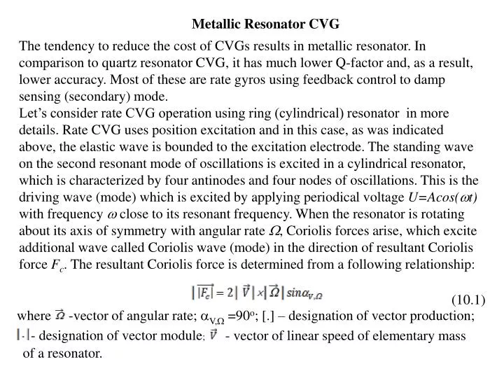
1. Metallic Resonator CVG The tendency to reduce the cost of CVGs results in metallic resonator. In comparison to quartz resonator CVG, it has much lower Q-factor and, as a result, lower accuracy. Most of these are rate gyros using feedback control to damp sensing (secondary) mode. Let’s consider rate CVG operation using ring (cylindrical) resonator in more details. Rate CVG uses position excitation and in this case, as was indicated above, the elastic wave is bounded to the excitation electrode. The standing wave on the second resonant mode of oscillations is excited in a cylindrical resonator, which is characterized by four antinodes and four nodes of oscillations. This is the driving wave (mode) which is excited by applying periodical voltage U=Acos(t) with frequency  close to its resonant frequency. When the resonator is rotating about its axis of symmetry with angular rate , Coriolis forces arise, which excite additional wave called Coriolis wave (mode) in the direction of resultant Coriolis force Fc. The resultant Coriolis force is determined from a following relationship: (10.1) where-vector of angular rate; V, =90o; [.] – designation of vector production; • - designation of vector module; - vector of linear speed of elementary mass of a resonator.

2. Antinode (Excitation) Excitation –Excitation (drive) signal Comp – Compensation signal Antinode – AntiNode signal Node – Node signal X Y a 1 Node (Comp) Node (Sense) 2 8 Antinode (Sense) 7 3 b Antinode (Sense) AntiNode (Sense) Excitation 4 Xout resonator Xin 6 Node (Sense) Node (Comp) 5 Comp Node (Sense) Antinode (Excitation) Yin Yout Thus, the Coriolis mode amplitude, excited by Coriolis forces is proportional to the angular rate . Differential equations describing the behavior of the two vibration modes (driving mode and Coriolis mode) can be represented as follows: (10.2) • Where x and y are the displacements along X (driving mode) and Y (Coriolis mode) axes (see fig.10.1a), respectively; x and y are the natural frequencies of driving and Coriolis modes of vibration; Qx and Qy are the quality factors of the vibration modes along X and Y axes; A is the Fig.10.1. Schematic of electrode disposition in cylindrical resonator • driving (excitation) force amplitude acting along X axis; k is Brian coefficient equal to about 0.4; is an angle rate measured.

3. Diametrically opposite electrodes (1-5; 2-6; 3-7; 4-8) are connected with each other, so that they have the same applied and sense voltages. As a result there are two output signals (sense) and two input signals (Excitation (drive) and Compensation) which are shown by “in” arrows and “out” arrows. It means that resonator as a plant is represented as a two-input-two-output control system,as shown in fig 10.1b. Coriolis mode amplitude is sensed by the piezoelectric electrode mounted on the nodal point of the driving wave and with the aid of feedback loop is suppressed by applying antipodal voltage on the one of the other of four nodes. So, feedback signal amplitude that compensates for the nodal vibration is proportional to angle rate . This measurement method, using compensated signal, is called compensated measurement method and is often used in practice.Linear velocity V of the resonator’s mass points is: =dU/dt=V=-Axsin(xt), where  is coefficient of proportionality between applied to resonator voltage and responded mechanical vibration amplitude. In order to make Fc = kproportional to , parameters A and xshould be constants. But x (resonant frequency of resonator) is changing of temperature, so this parameter should be tracked and responded mechanical vibration amplitude (A) should be stabilized at prescribed value during angle rate measurements. So, eight electrodes should be used to measure signals necessary to calculate controls and to measure angle rate .

4. Excitation channel Resonant frequency tracking system (PLL) frequency S1 C1 S1 Resonator Excitation amplitude ADC Excitation to Excitation DAC Band Pass filter Demodulator #1 Regulator #1 X С1 Ao GYRO out =SF Sense channel S1 Demodulator #2 Regulator #2 Compensation C1 Coriolis sub-channel Y to Compensation Band Pass filter 4 Quadrature sub-channel S1 Demodulator #3 Regulator #3 C1 Quadrature amplitude Fig.10.2. CVG control system block functional diagram These electrodes are located at all four antinodal and four nodal points of the resonator standing wave. It should be noted that all signals coming from resonator are amplitude modulated ones. The resonantfrequency is a carrier frequency (4-6 kHz) and angle rate  is modulating signal. In order to calculate controls, first of all demodulation should be carried out. In order to apply control signals to the resonator, modulation using resonant frequency should be carried out. CVG control system block functional diagram is presented in fig. 10.2.

5. Frequency meter  C1 + sin Antinode signal S1 Demodulator Regulator 2ТК Mod2 cos + C1 NCO DAC is a digital-to-analog converter; ADC is a analog-to-digital converter; Ao –Desired antinode amplitude.  is digital band-pass filter with central frequency equal to resonant frequency. It is used to reduce input noise and to pass useful signal. Resonant frequency tracking system is a digital phase lock loop (PLL) with numerically control oscillator (NCO) implemented in software. This system provides resonator changing frequency tracking and synthesizes reference signals С1, S1 to use them for demodulation and re-modulation of the control signals. Block diagram of the resonant frequency tracking system is presented in fig.10.3. Band Pass filter • Fig.10.3. Resonant frequency tracking system (PLL) • Mod2 - division by module 2; T– sample frequency (10-20s); K-PLL amplification coefficient (choose during adjustment); NCO – numerically controlled oscillator.

6. Multiplier Low Pass filter Carrier (resonant frequency) Envelope (angle rate,) Demodulator: it implements multiplication of input signal by reference one and low pass filtration to suppress high frequencies components arising after multiplication to separate low frequency envelope (see fig.10.4). Input signal is amplitude modulated signal as shown in fig.10.5. Reference signal Input signal Fig.10.4. Demodulator Fig.10.5. Amplitude modulated signal In general case the amplitude modulated signal can mathematically be described as follows: y(t)= [A+m(t)sin(mt+m)]sin(ct+c) ; t=it ;i=1…N, (10.3) where m – modulating frequency; c – carrier frequency; m, c– modulating and carrier signals phases, respectively. In expression (6.3) the next inequality should be valid m<<c and m(t) A. The ratio max(m)/A is called modulation index and expressed in percents. In case of CVG A=0, because in nodal point where angle rate arises the signal in absent of angle rate is equal to zero. When the resonator is rotating about its axis of symmetry with angle rate osin(t+),where o is angle rate amplitude, is

7. Angle rate signal spectrum S Modulated signal spectrum Amplitude frequency Characteristic of the low pass filter   2x- 2x+ angle rate frequency, is angle rate phase, the nodal signal is: y(t)= osin(t+)sin(xt) ; (10.4) here x is resonant frequency along X axis. Demodulation process is that to separate the low frequency envelope osin(t+), that is angle rate, from the high frequency carrier sin(xt) by multiplication the signal y(t) by the carrier frequency, which is reference signal (normalized antinode sense signal): y(t)sin(xt)= osin(t+)sin2(xt)= osin(t+)[1-cos(2xt)]/2= o sin(t+)/2-o sin(t+) cos(2xt)]/2= o sin(t+)/2-o sin[(2x+)t+]-sin[(2x-)t-]/2; (10.5) So, the first summand osin(t+)/2 multiplied by 2 is envelope (for CVG it is angle rate) and is concentrated at the low frequency  (usually 100Hz), the two others summands are concentrated at the double resonance frequencies 2x+ and 2x - (usually 2x10kHz). The power spectrum of the signal y(t)sin(xt) is shown in fig.10.6: Fig.10.6. Power spectrums of modulated and demodulated signals.

8. Kp + Input signal + Output signal + Kp + Output signal Input signal + When this signal is passing through the low pass filter with cut frequency a little more than, on the output of this filter only envelope o sin(t+)/2 can be obtained. Regulator: Proportional + integral (PI) regulators are used in this control system. PI regulator schematic in digital form is depicted in fig.10.7. Kp, KI are amplification coefficients of proportional and integral units, respectively. These coefficients should be chosen during control system adjustment. Fig.10.7. Proportional and integral (PI) regulator. • These coefficients define band pass of each loop and accuracy of the control loops. The values of these coefficients depend on the properties of the plant (resonator). • The digital PI regulator is a partial case of the very popular in practice proportional, integral and differential (PID) regulator is shown in fig.10.8. Fig.10.8. Proportional, integral and differential (PID) regulator.

9. The control system works as follows: Excitation channel  Antinode signal is provided to ADC (fig.10.4) and then to band pass filter to separate frequency band around resonant frequency x and to suppress any noise outside this band. After suppressing the noise the signal is divided by two branches with different components, sine and cosine components. Sine component is responsible for excitation amplitude control and cosine component – for phase control. Amplitude Control Sine component of the antinode signal is extracted by the demodulator #1 in view of stable vibration amplitude A0 which is set at discriminator. The error signal, difference between real amplitude of vibration and desirable one (A0) is provided to the regulator # 1, which gives the signal at its output so that to drive to null the signal at its input, that is to drive the vibration amplitude to A0. The regulator # 1 output signal is DC signal which should be re-modulated (modulated again) by multiplying by cosine component to send it to DAC and then in analog form (voltage) to drive (excitation) electrode.

10. Amplitude frequency characteristic Phase frequency characteristic Phase Ampl 90o+ 90o 90o- x  Fig.10.9. Resonator AFC and PhFC Phase Control (PLL) After antinode band pass filter the second branch of the antinode signal is provided to the PLL demodulator (see fig.10.3) and frequency meter. Cosine component of the antinode signal is extracted by the PLL demodulator which is proportional to the phase difference  between reference signal C1=cos(xt) and antinode signal: =A0 sin(xt+)cos(xt) = A0sin(xt++xt)+ A0sin(xt+-xt)= A0sin(2xt+)+ A0sin; after low pass filter = A0sinA0 , <<1; The signal  proportional to phase difference as an error signal is provided to PLL regulator which, after normalization to sample time T0 and amplification K times changes the frequency of numerically controlled oscillator (NCO) (equivalent to voltage controlled oscillator in analog electronic) so that to null the error signal . PLL keeps the drive frequency at the resonance frequency x. From the resonator amplitude and phase frequency characteristic follows (see fig.10.9) that when the drive frequency is not equal to resonant frequency the phase of the PLL demodulator output signal is not equal to 90o, so there arises phase difference 

11. which is not equal to zero and the regulator gives the signal proportional to phase difference  to return the drive frequency to the resonance by driving to null the phase difference . Frequency meter measure signal period by the number N of intersections of zero level for time T and calculates the frequency by the formula x=2/N/T.