Download
1 / 16
180 likes | 290 Views
OMI/TOMS Surface UV Irradiance algorithm. N.A. Krotkov, Goddard Earth Sciences and Technology Center /UMBC J. Herman, P.K.Bhartia,NASA/GSFC Colin Seftor, Raytheon ITSS Co A.Arola, J.Kaurola, L.Koskinen, S.Kalliskota, P.Taalas, FMI A.Vasilkov, SSAI. 340/380 nm residue. 380 nm radiance.

E N D
OMI/TOMSSurface UV Irradiance algorithm N.A. Krotkov, Goddard Earth Sciences and Technology Center /UMBC J. Herman, P.K.Bhartia,NASA/GSFC Colin Seftor, Raytheon ITSS Co A.Arola, J.Kaurola, L.Koskinen, S.Kalliskota, P.Taalas, FMI A.Vasilkov, SSAI
340/380 nm residue 380 nm radiance Ozone, surf. Ref, SZA Absorbing aerosol correction Table of clear sky fluxes Table of rad vs cloud optical depth Algorithm Overview • Algorithm based on corrections to calculated clear-sky UV irradiance Cloud corrected: Clear sky flux OR Abs. Aerosol corrected: • FClear calculationprocedure based on table lookups
Addressing reviewers’ questions • Cloud parameters (cloud height, model, fraction etc)– small error “Different combinations of cloud parameters yield strikingly similar estimates of surface UV irradiance” [Soulen and Frederick JGR 1999], [Krotkov et al JGR 2001] • Update of the aerosol error budget • Non-absorbing aerosols (oceanic and sulfate -see next slides) • Absorbing aerosols in the free troposphere (dust and smoke – see next) • Boundary layer absorbing aerosols (urban and pollution) – work in progress • Snow correction - work in progress through the FMI • Need real-time discrimination method between cloud and snow (from OMI cloud algorithm and/or ECWMF/DAO assimilation) • Validation • WMO Brewer network [Fioletov et al 2002], [McKenzie et al JGR 2001] • USA USDA network, oceanic environment – in progress
Quantifying errors due to non-absorbing aerosol Using radiative transfer calculations and OMI synthetic spectra we were able to confirm that C1 cloud model does not produce a bias for non-absorbing (oceanic and sulfate aerosols)
New parameterization for dust aerosol Using new AERONET aerosol models [Dubovik et al 2002] and OMI synthetic data we have come up with the new parameterizations for absorbing aerosol correction. The new correction reduces the error to +/-5% for dust aerosol if the dust altitude is known
Absorbing aerosols in free troposphere (dust, smoke) can be corrected using Aerosol Index method Industrial aerosols close to the ground remain a major challenge: neither correction method works well
Largest bias (+20%- 40%) was found for industrial and mountain sites in Europe +10% average bias for 10 Canadian Brewer sites no bias for clean sites Several groups has compared TOMS UV data with ground UV measurements [McKenzie et al JGR 2001, Fioletov et al, SPIE 2001]
Industrial aerosols reduce UV up to 30% Cloud correction overestimates surface UV in the presence of industrial aerosols up to 20% Aerosol Index (AI) correction is not applied since AI < 0
The aerosol error can be corrected locally if UV aerosol climatology is known To correct for industrial aerosols one has to know both UV optical thickness AND UV single scattering albedo
TOMS UV algorithm is being validated using Brewer ground measurements [Fioletov et al 2002] TOMS can successfully reproduce long-term and major short term UV variations, although there are some systematic differences. The bias can be seen at clear sky conditions and at 324nm, i.e. it is not related to local cloud conditions or absorption by ozone and SO2 Daily CIE irradiation measured by Brewer and estimated from TOMS at Toronto in May-June 2000. The correlation coefficient between the measured and derived from TOMS irradiation plotted here is 0.9. The standard deviation of the difference between the measured and derived UV is about 16%.
Table 1. Summer (June-August for Churchill and May-August for all other) Noon CIE Irradiation Statistics for Brewer Stations.
Interannual relative changes in estimated and measured UV irradiance (1979-2000) March Annual average
On-going work • we have been successfully working to overcome the differences between ground-based and satellite estimations. • Useful improvements will be implemented in the second version of the UV algorithm which will be shared between TOMS, OMI, GOME and TRIANA/EPIC UV products. • The previous TOMS data record (since 1978) will be re-processed with the improved UV algorithm to ensure homogeneity of the combined satellite global UV record for the future trend analysis.
Surface/snow albedo correction TOMS 380nm Monthly Minimum LER (MLER) [Herman and Celarier 1997]
Cooperation with FMI: work in progress on new method of snow correction Arola et al, JGR 2002