One Tailed and Two Tailed tests

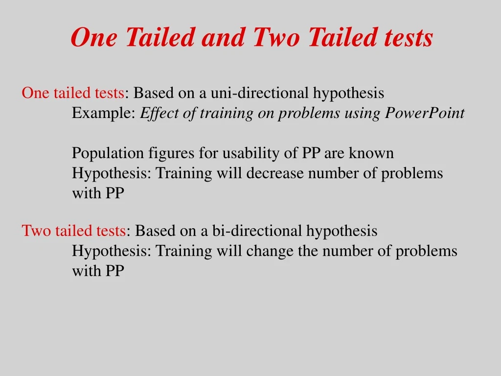
1. One Tailed and Two Tailed tests One tailed tests: Based on a uni-directional hypothesis Example: Effect of training on problems using PowerPoint Population figures for usability of PP are known Hypothesis: Training will decrease number of problems with PP Two tailed tests: Based on a bi-directional hypothesis Hypothesis: Training will change the number of problems with PP

2. Sampling Distribution Population for usability of Powerpoint 1400 1200 1000 800 Frequency 600 400 Std. Dev = .45 200 Mean = 5.65 N = 10000.00 0 3.75 4.75 5.25 6.25 7.00 7.25 4.00 4.25 4.50 5.00 5.50 5.75 6.00 6.50 6.75 Mean Usability Index If we know the population mean Identify region Unidirectional hypothesis: .05 level Bidirectional hypothesis: .05 level

3. What does it mean if our significance level is .05? • For a uni-directional hypothesis • For a bi-directional hypothesis PowerPoint example: • Unidirectional • If we set significance level at .05 level, • 5% of the time we will higher mean by chance • 95% of the time the higher mean mean will be real • Bidirectional • If we set significance level at .05 level • 2.5 % of the time we will find higher mean by chance • 2.5% of the time we will find lower mean by chance • 95% of time difference will be real

4. Changing significance levels • What happens if we decrease our significance level from .01 to .05 • Probability of finding differences that don’t exist goes up (criteria becomes more lenient) • What happens if we increase our significance from .01 to .001 • Probability of not finding differences that exist goes up (criteria becomes more conservative)

5. PowerPoint example: • If we set significance level at .05 level, • 5% of the time we will find a difference by chance • 95% of the time the difference will be real • If we set significance level at .01 level • 1% of the time we will find a difference by chance • 99% of time difference will be real • For usability, if you are set out to find problems: setting lenient criteria might work better (you will identify more problems)

6. Effect of decreasing significance level from .01 to .05 • Probability of finding differences that don’t exist goes up (criteria becomes more lenient) • Also called Type I error (Alpha) • Effect of increasing significance from .01 to .001 • Probability of not finding differences that exist goes up (criteria becomes more conservative) • Also called Type II error (Beta)

7. Degree of Freedom • The number of independent pieces of information remaining after estimating one or more parameters • Example: List= 1, 2, 3, 4 Average= 2.5 • For average to remain the same three of the numbers can be anything you want, fourth is fixed • New List = 1, 5, 2.5, __ Average = 2.5

8. Major Points • T tests: are differences significant? • One sample t tests, comparing one mean to population • Within subjects test: Comparing mean in condition 1 to mean in condition 2 • Between Subjects test: Comparing mean in condition 1 to mean in condition 2

9. Effect of training on Powerpoint use • Does training lead to lesser problems with PP? • 9 subjects were trained on the use of PP. • Then designed a presentation with PP. • No of problems they had was DV

10. Powerpoint study data • Mean = 23.89 • SD = 4.20

11. Results of Powerpoint study. • Results • Mean number of problems = 23.89 • Assume we know that without training the mean would be 30, but not the standard deviation Population mean = 30 • Is 23.89 enough larger than 30 to conclude that video affected results?

12. Sampling Distribution of the Mean • We need to know what kinds of sample means to expect if training has no effect. • i. e. What kinds of means if m = 23.89 • This is the sampling distribution of the mean.

13. Sampling Distribution of the Mean--cont. • The sampling distribution of the mean depends on • Mean of sampled population • St. dev. of sampled population • Size of sample

14. Sampling Distribution Number of problems with Powerpoint Use 1400 1200 1000 800 Frequency 600 400 Std. Dev = .45 200 Mean = 5.65 N = 10000.00 0 3.75 4.00 4.25 4.50 4.75 5.00 5.25 5.50 5.75 6.00 6.25 6.50 6.75 7.00 7.25 Mean Number of problems Cont.

15. Sampling Distribution of the mean--cont. • Shape of the sampled population • Approaches normal • Rate of approach depends on sample size • Also depends on the shape of the population distribution

16. Implications of the Central Limit Theorem • Given a population with mean = m and standard deviation = s, the sampling distribution of the mean (the distribution of sample means) has a mean = m, and a standard deviation = s /n. • The distribution approaches normal as n, the sample size, increases.

17. Demonstration • Let population be very skewed • Draw samples of 3 and calculate means • Draw samples of 10 and calculate means • Plot means • Note changes in means, standard deviations, and shapes Cont.

18. Parent Population Cont.

19. Sampling Distribution n = 3 Cont.

20. Sampling Distribution n = 10 Cont.

21. Demonstration--cont. • Means have stayed at 3.00 throughout--except for minor sampling error • Standard deviations have decreased appropriately • Shapes have become more normal--see superimposed normal distribution for reference

22. One sample t test cont. • Assume mean of population known, but standard deviation (SD) not known • Substitute sample SD for population SD (standard error) • Gives you the t statistics • Compare t to tabled values which show critical values of t

23. t Test for One Mean • Get mean difference between sample and population mean • Use sample SD as variance metric = 4.40

24. Degrees of Freedom • Skewness of sampling distribution of variance decreases as n increases • t will differ from z less as sample size increases • Therefore need to adjust t accordingly • df = n - 1 • t based on df

25. Looking up critical t (Table E.6)

26. Conclusions • Critical t= n = 9, t.05 = 2.62 (two tail significance) • If t > 2.62, reject H0 • Conclude that training leads to less problems

27. Factors Affecting t • Difference between sample and population means • Magnitude of sample variance • Sample size

28. Factors Affecting Decision • Significance level a • One-tailed versus two-tailed test