Download
1 / 10
160 likes | 482 Views
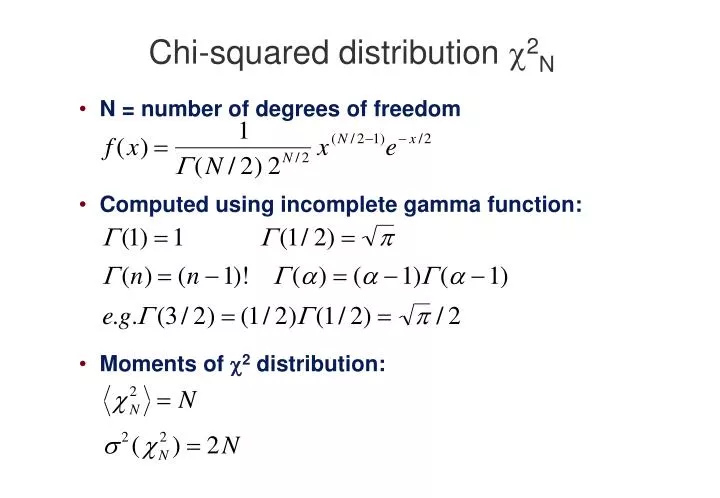
Chi-squared distribution 2 N. N = number of degrees of freedom Computed using incomplete gamma function: Moments of 2 distribution:. Constructing 2 from Gaussians - 1. Let G(0,1) be a normally-distributed random variable with zero mean and unit variance. For one degree of freedom:

E N D
Chi-squared distribution 2N • N = number of degrees of freedom • Computed using incomplete gamma function: • Moments of 2 distribution:
Constructing 2 from Gaussians - 1 • Let G(0,1) be a normally-distributed random variable with zero mean and unit variance. • For one degree of freedom: • This means that: -a a i.e. The 2 distribution with 1 degree of freedom is the same as the distribution of the square of a single normally distributed quantity. G(0,1) a2 21
X2 X1 Constructing 2 from Gaussians - 2 • For two degrees of freedom: • More generally: • Example: Target practice! • If X1 and X2 are normally distributed: • i.e. R2 is distributed as chi-squared with 2 d.o.f
Data points with no error bars • If the individual i are not known, how do we estimate for the parent distribution? • Sample mean: • Variance of parent distribution: • By analogy, define sample variance: • Is this an unbiased estimator, i.e. is <s2>=2?
Estimating 2 – 1 • Express sample variance as: • Use algebra of random variables to determine: • Expand: (Don’t worry, all will be revealed...)
X <X> Xi <Xi> Aside: what is Cov(Xi,X)?
Estimating 2 – 2 • We now have • For s2 to be an unbiased estimator for 2, need A=1/(N-1):
Degrees of freedom – 1 <X> • If all observations Xi have similar errors : • If we don’t know <X> use X instead: • In this case we have N-1 degrees of freedom. Recall that: • (since <2N>=N)
Degrees of freedom – 2 • Suppose we have just one data point. In this case N=1 and so: • Generalising, if we fit N data points with a function A involving M parameters 1... M: • The number of degrees of freedom is N-M.
Example: bias on CCD frames • Suppose you want to know whether the zero-exposure (bias) signal of a CCD is uniform over the whole image. • First step: determine s2(X) over a few sub-regions of the frame. • Second step: determine X over the whole frame. • Third step: Compute • In this case we have fitted a function with one parameter (i.e. the constant X), so M=1 and we expect < 2 > = N - 1 • Use 2N - 1 distribution to determine probability that 2> 2obs