Download
1 / 27
270 likes | 488 Views
Dealing with NP-Complete Problems. Roman Ginis Mani Chandy. What to do with NP-Complete Problems?. Good sense (and humility) suggest that we probably can’t find algorithms that take polynomial time in the worst case for NP-complete problems.

E N D
Dealing with NP-Complete Problems Roman Ginis Mani Chandy
What to do with NP-Complete Problems? • Good sense (and humility) suggest that we probably can’t find algorithms that take polynomial time in the worst case for NP-complete problems. • Because if we did find a polynomial solution to an NP-complete problem then P = NP, and we have found polynomial solutions for all problems in NP.
What to do with NP-Completeness? • Worst case solutions may be exponential but solution may take only polynomial time on the average. • Fast average time solutions are good, but in many cases we don’t have fast average time solutions either.
What to do? • Find solutions that work well much of the time, even if we can’t prove that average solution time is fast. • Find solutions that are within specified bounds of the optimal. Example: You are looking for any solution to a traveling salesman problem which is provably within 20% of optimal.
An Approach: Branch and Bound • An example: the knapsack problem. • Recall what the knapsack problem is: • Given a knapsack with capacity C • Given N objects, where the j-th object has weight W[j] and value V[j]. • Put objects into knapsack to maximize value of knapsack contents without exceeding its capacity.
0 - 1 Knapsack Problem • Assume that all parameters (capacity, values, weights) are positive integers. • Mathematical formulation • max (sum over all j of V[j]*x[j]) • subject to (sum over all j of W[j]*x[j]) <= C • where x[j] is 0 or 1 • x[j] = 1 if and only if the object is placed in the knapsack.
Branch and Bound for Knapsack • The Knapsack Problem is NP-Complete. • Suppose we want to find a solution within 20% of optimal, or • We want to run an algorithm for 2 days and then pick the best solution we have found so far, and we’d like the algorithm to tell us that it is within P% of the optimal solution where P is determined by the algorithm.
Bounds • If we are maximizing, and we have a solution with value V, and we want to prove that this solution is within 20% of the optimal, then we can do so by proving that V is within 20% of an upper bound to the optimal solution. • Maximizing --- find upper bound • Minimizing --- find lower bound
Finding bounds • One way: relax the constraints. • Suppose the given problem is Z = max f(x) subject to x in set B. • We relax the constraint by requiring x to be in a set D, where B is contained in D. • The relaxed problem is Z’ = max f(x) subject to x in set D. • What is the relationship between Z and Z’?
Relaxing Constraints B Z is the best solution in set B D Z’ is the best solution in set D B
Solutions to Relaxed Problems • The optimal solution to a relaxed problem is at least as good as the optimal solution to the original problem because an optimal solution to the original problem is also a feasible solution to the relaxed problem. • So we get bounds by relaxing constraints: • maximizing: upper bounds • minimizing: lower bounds
Finding Bounds • We want tight bounds because the tighter the bounds the smaller the amount we can claim our solution is from the optimal. • Example: We have a feasible solution with value 100 and our upper bound is 110, so we know that the optimal solution is within 10% of the optimal. What can we claim if our bound is 200?
Finding bounds • We want to compute bounds quickly because, as we shall see shortly, we will be computing bounds repeatedly. • We have to evaluate the tradeoff between computing very tight bounds and computing bounds rapidly, and there is no obvious way of doing this.
Bounds for Knapsack • We find a bound for the knapsack problem by relaxing its constraints. • One way to relax constraints is to relax the requirement that objects are indivisible. • In the given problem you are not allowed to put a fraction of an object into a knapsack. • In relaxed problem fractional objects are ok.
Bounds for Knapsack • Given problem • max (sum over j of V[j]*x[j]) • subject to (sum over j of W[j]*x[j]) <= C • x[j] = 0 or 1. • Relaxed problem • same as given problem except: 0 <= x[j] <= 1
The Cheesecake Problem • The relaxed knapsack problem is called the cheesecake problem. Why? • How would you solve the cheesecake problem fast?
The Cheesecake Name • It’s called the cheesecake problem because you can think of the knapsack as your stomach, and the objects as cheesecakes. • A value of a cheesecake is the pleasure you get out of eating it. • The weight of a cheesecake is … well it’s weight.
Solutions to the Cheesecake • Order objects in decreasing value-density, i.e., by value divided by weight. Assume this ordering is 1, 2, 3,… the natural order. • The maximum happiness you get out of one bite (one gram) of a cheesecake is from cheesecake 1, then cheesecake 2, …. • Optimum solution: eat cheesecakes in order 1,2, 3, … until you can’t eat any more.
Solutions to Cheesecake • Go in increasing order of cheesecakes. • Initial weight of cheesecakes in stomach: 0. • If next cheesecake fits in stomach then eat it all else eat the fraction that fills stomach. • Proof of optimality? Any other solution can be shown to be non-optimal by perturbing it
The Solution Tree We can represent all solutions to the knapsack problem as a tree. (Remember the trees we constructed to describe solutions by non-deterministic Turing machines?) root X[1] = 0 X[1] = 1 X[2] = 1 X[2]=0 X[2]= 1 X[2] = 0 X[3]=0 X[3]=1 X[3]=0 X[3]=1 X[3]=0 X[3]=1 X[3]=0 X[3]=1 001 010 011 100 101 110 111 000
The Solutions Tree • We construct the tree by making a decision about the value of x[j] for some j, setting the value to 0 or to 1. • At each level of the tree we set the value of the same variable x[j]. • There are 2n leaves of the tree, so generating the whole tree will definitely take exponential time.
A Brute Force Approach • Generate the whole solutions tree. • Each leaf corresponds to a solution (which may not be feasible because the total weight exceeds capacity). • If a solution is infeasible, discard it. • Keep track of the best feasible solution seen so far.
Central Question • Is there some way to find an optimal solution, or a solution that is guaranteed to be within a specified percentage of optimal, without generating the whole tree? • Is there some way to use bounds to keep the tree “pruned?”
The Approach • As we generate the tree, we will compute an upper bound for each node of the tree. • Bound associated with a node is an upper bound on all solutions that can be generated by expanding that node of the tree. • A feasible solution that is at least as good as the best bound is an optimal solution, as we shall see.
Tree Generations • Suppose V = [7, 5, 3] • W = [6, 5, 4] • C = 9 • Can we use bounds to get better solutions?
The Solution Tree Which node of the tree should we expand next? root X[1] = 0 X[1] = 1 infeasible X[2] = 1 X[2]=0 X[2]= 1 X[2] = 0 Bound = - infinity Bound =3 Bound = 8 X[3]=0 X[3]=1 Bound = 7 Bound = - infinity
The Central Idea • Always expand that leaf of the (partially-expanded) tree with the best bound. • Note: An upper bound on the optimal solution is the minimum value of the bounds associated with all the leaves of the partially-expanded tree. More next class.