Download
1 / 72
720 likes | 884 Views
Chapter 14: Elements of Nonparametric Statistics. Chapter Goals. Introduce the basic concepts of nonparametric statistics, or distribution-free techniques. Nonparametric statistics are versatile and easy to use. Consider some of the most common tests and applications.

E N D
Chapter Goals • Introduce the basic concepts of nonparametric statistics, or distribution-free techniques. • Nonparametric statistics are versatile and easy to use. • Consider some of the most common tests and applications.
14.1: Nonparametric Statistics • Parametric methods: Assume the population is at least approximately normal, or use the central limit theorem. • Nonparametric methods, or distribution-free methods: Assume very little about the population, subject to less confining restrictions.
Nonparametric statistics have become popular: 1. Require few assumptions about the underlying population. 2. Generally easier to apply than their parametric counterparts. 3. Relatively easy to understand. 4. Can be used in situations where the normality assumptions cannot be made. 5. Generally only slightly less efficient than their parametric counterparts. Disadvantages?
14.2: Comparing Statistical Tests • Four nonparametric tests presented in this chapter. There are many others. • Many nonparametric tests may be used as well as certain parametric tests. • Which statistical test is appropriate: the parametric or nonparametric.
Which test is best? 1. When comparing two tests they must be equally qualified for use; they must both be appropriate test procedures. 2. Each test has a set of assumptions that must be satisfied. 3. The best test: The test that is best able to control the risks of error and at the same time keeps the sample size reasonable. 4. A larger sample size usually means a higher cost.
The Risk of Error: 1. Type I Error: Controlled directly (set) by the level of significance a. 2. P(type I error) = a, P(type II error) = b 3. We try to control b. 4. The power of a statistical test = 1 -b The power of a test is the probability that we reject the null hypothesis when it is false (a correct decision). If two appropriate statistical tests have the same significance level a, the one with the greater power is better.
The sample size: 1. Set acceptable values for a and b. Determine the sample size necessary to satisfy these values. 2. The statistical test that requires the smaller sample size is better. 3. Efficiency: The ratio of the sample size of the best parametric test to the sample size of the best nonparametric test when compared under a fixed set of risk values. Example: Efficiency rating for the sign test is approximately 0.63. This means that a sample of size 63 with a parametric test will do the same job as a sample of size 100 for the sign test.
To determine the choice of test: 1. Often forced to use a certain test because of the nature of the data. 2. When there is a choice, consider three factors: a. The power of the test. b. The efficiency of the test. c. The data (and the sample size). Note: The following table shows a comparison of nonparametric tests (presented in this chapter) with the parametric tests presented earlier.
14.3: The Sign Test • Versatile, easy to apply, uses only plus and minus signs. • Three sign test applications: confidence interval for a median, hypothesis test concerning a median, hypothesis test concerning the median difference (paired difference) for two dependent samples.
Assumptions for inferences about the population median using the sign test: The n random observations forming the sample are selected independently and the population is continuous in the vicinity of the median, M. Procedure for using the sign test to obtain a confidence interval for an unknown population median, M: 1. Arrange the data in ascending order (smallest to largest): x1 (smallest), x2, x3, . . . , xn (largest) 2. Use Table 12, Appendix B to obtain the critical value, k (the maximum allowable number of signs). 3. k indicates the number of positions to be dropped from each end of the ordered data. 4. The remaining extreme values are the bounds for a 1 -a confidence interval. Confidence Interval: xk+1 to xn-k Note: Based on the binomial distribution.
Example: Suppose 20 observations are selected at random and are given in ascending order (x1, x2, x3, . . . , x20). 19 21 23 28 31 32 33 34 34 35 38 41 43 43 44 46 47 48 52 55 Find a 95% confidence interval for the population median. Solution: Table 12: n = 20, a = 0.05 Þ k = 5 Drop the last 5 values on each end. The confidence interval is bounded by x6 and x10. The confidence interval: 32 to 44 (inclusive). In general: xk+1 to xn-kis a 1 -a confidence interval for M.
Single-Sample Hypothesis Test Procedure: 1. The sign test may be used when the null hypothesis concerns the population median M. 2. The test may be either one- or two-tailed. Example: A random sample of 88 tax payers was selected and each was asked the amount of time spent preparing their federal income tax return. Test the hypothesis “the median time required to prepare a return is 8 hours” against the alternative that the median is greater than 8 hours. The data is summarized by: Under 8: 37; Equal 8: 3; Over 8: 48 Use the sign test with a = 0.025.
Solution: The data is converted to (+) and (-) signs according to whether the data is more or less than 8. A plus sign is assigned to each observation greater than 8. A minus sign is assigned to each observation less than 8. A zero is assigned to each observation equal to 8. The sign test uses only the plus and minus signs. The zeros are discarded. Usable sample size = 88 - 3 = 85 n(+) = 48 n(-) = 37 n(+) +n(-) = n = 85
1. The Set-up: a. Population parameter of concern: M, population median time to prepare a federal income tax return. b. The null and alternative hypothesis: H0: M = 8 Ha: M > 8 2. The Hypothesis Test Criteria: a. Assumptions: The 88 observations were randomly selected and the variable time to prepare a return is continuous. b. Test statistic: x = the number of the less frequent sign = n(-) c. Level of significance: a = 0.025
3. The Sample Evidence: n = 85; x = n(-) = 37 4. The Probability Distribution (Classical Approach): a. Critical value: The critical region is one-tail. Table 12 is for two-tailed tests. At the intersection of the column a = 0.05 (= 2 ´ 0.025) and the row n = 85: k = 32. The critical value: k = 32. b. x is not is the critical region.
4. The Probability distribution (p-Value Approach): a. The p-value: Using Table 12: P > (0.25/2) = 0.125 Using a computer: P = 0.1928 b. The p-value is larger than the level of significance, a. 5. The Results: a. Decision: Do not reject H0. b. Conclusion: At the 0.025 level of significance, there is no evidence to suggest the median time required to complete a federal income tax return is greater than 8 hours.
Two Sample Hypothesis Test Procedure: 1. The sign test may also be used in tests concerning the median difference between paired data that result from two dependent samples. 2. A common application: the use of before-and-after testing to determine the effectiveness of some activity. 3. The signs of the differences are used to carry out the test. Zeros are discarded. Assumptions for inferences about median of paired differences using sign test:The paired data is selected independently and the variables are ordinal or numerical.
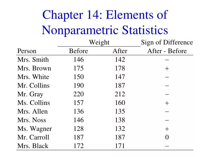
Example: A new automobile engine additive (included during an oil change) is designed to decrease wear and improve engine performance by increasing gas mileage. Sixteen randomly selected automobiles were selected and the before-and-after miles per gallon were recorded. (The same driver was used before and after the engine treatment.) Is there any evidence to suggest the engine additive improves gas mileage? Use a = 0.05. Note: The claim being tested is that the additive improves gas mileage. Form all the differences, After - Before. We will only reject the null hypothesis if there are significantly more plus signs.
1. The Set-up: a. Population parameter of concern: M, median gain in miles per gallon. b. The null and alternative hypothesis: H0: M = 0 (no mileage gain) Ha: M > 0 (mileage gain) 2. The Hypothesis Test Criteria: a. Assumptions: The automobiles were randomly selected and the variables, miles per gallon before and after, are both continuous. b. Test statistic: The number of the less frequent sign. In this example: x = n(-) c. Level of significance: 0.05
3. The Sample Evidence: n = 16; n(+) = 10; n(-) = 6 Observed value of the test statistic: x = n(-) = 6 4. The Probability Distribution (Classical Approach): a. Critical Value: The critical region is one-tail. Table 12 is for two-tailed tests. At the intersection of the column a = 0.10 (= 2 ´ 0.05) and the row n = 16: k = 4. The critical value: k = 4. b. x is not in the critical region.
4. The Probability Distribution (p-Value Approach): a. The p-value: Using Table 12: P > (0.25/2) = 0.125 Using a computer: P = 0.2272 b. The p-value is larger than the level of significance, a. 5. The Results: a. Decision: Do not reject H0. b. Conclusion: At the 0.05 level of significance, there is no evidence to suggest the engine additive increases the miles per gallon.
Normal Approximation: 1. The sign test may be carried our using a normal approximation and the standard normal variable z. 2. The normal approximation is used if Table 12 does not show the desired level of significance or if n is large. Procedure: 1. x is the number of the less frequent sign or the most frequent sign; consistent with the alternative hypothesis. 2. x is a binomial random variable with p = 0.5.
3. x is a binomial random variable, but it does become approximately normal for large n. Problem: A binomial random variable is discrete and a normal random variable is continuous. Solution: Use the continuity correction: an adjustment in the normal random variable so that the approximation is more accurate. Continuity Correction: a. For the binomial random variable, the area of a rectangular bar represents probability: width 1, from 1/2 unit below to 1/2 unit above the value of interest. b. When z is used, make a 1/2 unit adjustment before calculating the observed value of z. c. x’ is the adjusted value for x. If x > n/2 then x’ = x- (1/2) If x < n/2 then x’ = x+ (1/2)
Continuity Correction Illustration: P(x = 7) » P(6.5 £x£ 7.5) continuous discrete
1 -a confidence interval for M: Using the normal approximation (including the continuity correction), the position numbers are: The interval is xL to xU where Note: L should be rounded down and U should be rounded up to be sure the level of confidence is at least 1 -a.
Example: Estimate the population median with a 95% confidence interval for a given data set with 55 observations: x1, x2, x3, . . . , x54, x55. Solution: The position numbers are: L = 27.5 - 7.77 = 19.73; rounded down, L = 19. U = 27.5 + 7.77 = 35.27; rounded up, U = 36. Therefore: 95% confidence interval for M: x19 to x36.
Hypothesis test concerning M: Using the standard normal distribution, z is computed using the formula: Example: In a recent study children between the ages of 8 and 12 were reported to watch a median of 18 hours of television per week. In order to test this claim, 105 children between 8 and 12 were selected at random and the number of hours of television watched per week were recorded. A plus sign was coded if the number of hours was greater than 18, a minus sign if less than or equal to18: there were 71 plus signs and 34 minus signs. Use the normal approximation to the sign test to determine if there is any evidence to suggest the median number of hours watched is greater than 18. Use a = 0.05
Solution: 1. The Set-up: a. Population parameter of concern: M, the median number of hours of television watched per week. b. The null and alternative hypothesis: H0: M = 18 (£) (at least as may minus signs as plus signs) Ha: M > 18 (fewer minus signs than plus signs) 2. The Hypothesis Test Criteria: a. Assumptions: The random sample of 105 students was independently surveyed and the variable, hours of television watched per week, is continuous. b. Test statistic: z* c. Level of significance: a = 0.05
3. The Sample Evidence: a. Sample information: n(+) = 71, n(-) = 34 n = 105 and x = 71 b. Calculate the value of the test statistic: 4. The Probability Distribution (Classical Approach): a. Critical value: z(0.05) = 1.65 b. z* is in the critical region.
4. The Probability Distribution (p-Value Approach): a. The p-value: P = P(z* > 3.51) » 0.0002 Using a computer: P» 0.000224 b. The p-value is smaller than the level of significance, a. 5. The Results: a. Decision: Reject H0. b. Conclusion: At the 0.05 level of significance, there is evidence to suggest the median number of hours of television watched per week is greater than 18.
14.4: The Mann-Whitney U Test • Nonparametric alternative for the t test for the difference between two independent means. • Null hypothesis: the two sampled populations are identical.
Assumptions for inferences about two populations using the Mann-Whitney test: The two independent random samples are independent within each sample as well as between samples, and the random variables are ordinal or numerical. Note: 1. This test procedure is often applied in situations in which the two samples are drawn from the same population of subjects, but different treatments are used on each sample. 2. Test procedure described in the following example.
Example: A recent study claimed that adults who exercise regularly tend to have lower pulse rates. To test this claim, two independent random samples of adult males were selected, one from those who exercise regularly (A), and one from those who are more sedentary (B). The data is given below. Is there any evidence to suggest that adults who exercise regularly have lower pulse rates than those who do not exercise regularly. Use a = 0.05.
Solution: 1. The Set-up: a. Population parameter of concern: The distribution of pulse rates for each population of adult males. b. The null and alternative hypothesis: H0: Populations A and B have pulse rates with identical distributions. Ha: The two distributions are not the same. 2. The Hypothesis Test Criteria: a. Assumptions: The two samples are independent, and the random variable (pulse rate) is numerical. b. Test statistic: Mann-Whitney U Statistic, described below. c. Level of significance: a = 0.05
3. The Sample Evidence: a. Sample information: Data given in the table above. b. Calculate the value of the test statistic: na = sample size from population A nb = sample size from population B Combine the two samples and order the data from smallest to largest. Assign each observation a rank number. The smallest observation is assigned rank 1, the next smallest is assigned rank 2, etc., up to the largest, which is assigned rank na+nb. For ties: assign each of the tied observations the mean rank of those rank positions that they occupy.
To Compute the U Statistic: 1. Compute the sum of the ranks for each of the two samples: Ra and Rb. 2. Compute the U score for each sample: 3. The test statistic, U*, is the smaller of Ua and Ub.
Background: 1. Suppose the two samples are very different. Small ranks are associated with one sample, large ranks with the other. U* would tend to be small, and we would want to reject the null hypothesis. 2. Suppose the two samples are very similar. The ranks are evenly distributed between the two samples. Ua and Ub tend to be about equal, U* tends to be larger. Note: Ua+Ub = na´nb Therefore: only need to consider the smaller U-value.
4. The Probability Distribution (Classical Approach): a. Critical value: Use Table 13B, one-tailed, a = 0.05 Critical value is at the intersection of column n1 = 10 and row n2 = 10: 27 b. U* is not in the critical region. 4. The Probability Distribution (p-Value Approach): a. The p-value: P = P(U* £ 30, for n1 = 10 and n2 = 10) Using Table 13: P > 0.05 Using a computer: P » 0.0694 b. The p-value is not smaller than a.
5. The Results: a. Decision: Do not reject H0. b. Conclusion: At the 0.05 level of significance, there is no evidence to suggest the two populations are different. Normal Approximation: If the sample sizes are large, then U is approximately normal with The standard normal distribution may be used if both sample sizes are greater than 10; the test statistic is
Example: The data below represents the number of hours two different cellular phone batteries worked before a recharge was necessary. Is there any evidence to suggest battery type B lasts longer than battery type A. Use the Mann-Whitney test with a =0.05.
Solution: 1. The Set-up: a. Population parameter of concern: The distribution of battery life for each brand. b. The null and alternative hypothesis: H0: The distributions for battery life are the same for both brands. Ha: The distributions are not the same. 2. The Hypothesis Test Criteria: a. Assumptions: The two samples are independent and the random variable, battery life, is continuous. b. Test statistic: Mann-Whitney U statistic (normal approximation). c. Level of significance: a = 0.05
3. The Sample Evidence: a. Sample information: Data given in the table above. b. Calculate the value of the test statistic: Rankings for battery life:
The sums: The U scores:
4. The Probability Distribution (Classical Approach): a. Critical value: -z(0.05) = -1.65 b. z* is not in the critical region. 4. The Probability Distribution (p-Value Approach): a. The p-value: P = P(z* < -.6101) = .2709 b. The p-value is not smaller than a. 5. The Results: a. Decision: Do not reject H0. b. Conclusion: At the 0.05 level of significance, there is no evidence to suggest the battery life for brand B is longer than the life for brand A.