Download
1 / 21
210 likes | 346 Views
Chapter 2. Linearization. Interacting Tank-in-Series System. Linearize the the interacting tank-in-series system for the operating point resulted by the parameter values as given in Homework 2. For q i , use the last digit of your Student ID. For example: Kartika q i = 8 liters/s.

E N D
Chapter 2 Linearization Interacting Tank-in-Series System Linearize the the interacting tank-in-series system for the operating point resulted by the parameter values as given in Homework 2. • For qi, use the last digit of your Student ID. For example: Kartika qi= 8 liters/s. • Submit the mdl-file and the screenshots of the Matlab-Simulink file + scope. qi h1 h2 q1 a1 a2 v1 v2
Chapter 2 Linearization Interacting Tank-in-Series System • The model of the system is: • As can be seen from the result of Homework 2, the steady state parameter values, which are taken to be the operating point, are:
Chapter 2 Linearization Interacting Tank-in-Series System • The linearization around the operating point (h1,0,h2,0,qi,0) is performed as follows:
Chapter 2 Linearization Interacting Tank-in-Series System
Chapter 2 Linearization Interacting Tank-in-Series System
Chapter 2 Linearization Interacting Tank-in-Series System
Chapter 2 Linearization Interacting Tank-in-Series System
Chapter 2 Linearization Interacting Tank-in-Series System : h1, original model : h2, original model : h1, linearized model : h2, linearized model
Chapter 2 Linearization Interacting Tank-in-Series System : h1, original model : h2, original model : h1, linearized model : h2, linearized model
Chapter 2 Linearization Interacting Tank-in-Series System : h1, original model : h2, original model : h1, linearized model : h2, linearized model
Chapter 3 Analysis of Process Models State Space Process Models • Consider a continuous-time MIMO system with m input variables and r output variables. The relation between input and output variables can be expressed as: : vector of state space variables : vector of input variables : vector of output variables
Chapter 3 State Space Process Models Solution of State Space Equations • Consider the state space equations: • Taking the Laplace Transform yields:
Chapter 3 State Space Process Models Solution of State Space Equations • After the inverse Laplace transformation, • The solution of state space equations depends on the roots of the characteristic equation:
Chapter 3 State Space Process Models Solution of State Space Equations Consider a matrix . Calculate .
Chapter 3 State Space Process Models Canonical Transformation • Eigenvalues of A, λ1, …, λn are given as solutions of the equation det(A–λI) = 0. • If the eigenvalues of A are distinct, then a nonsingular matrix T exists, such that: is a diagonal matrix of the form
Chapter 3 State Space Process Models Canonical Transformation • Example Perform the canonical transformation to the state space equations below • The eigenvalues of A
Chapter 3 State Space Process Models Canonical Transformation • The eigenvectors of A
Chapter 3 State Space Process Models Canonical Transformation The equivalence transformation can now be done, with x = Tx. Then, the state space equations ~ As the result, we obtain a state space in canonical form,
Chapter 3 Homework 4: Canonical Transformation State Space Process Models • Make yourself familiar with the canonical transformation. Obtain the canonical form of the state space below.
Chapter 3 Homework 4: Canonical Transformation State Space Process Models • Perform the canonical transformation for the following state space equation. NEW • Hint: Learn the following functions in Matlab: [V,D] = eig(X)