Download
1 / 28
280 likes | 362 Views
Lecture 13. Further with interferometry – Resolution and the field of view; Binning in frequency and time, and its effects on the image; Noise in cross-correlation; Gridding and its pros and cons. Earth-rotation synthesis. Apply appropriate delays: like measuring V

E N D
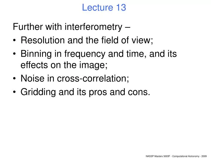
Lecture 13 Further with interferometry – • Resolution and the field of view; • Binning in frequency and time, and its effects on the image; • Noise in cross-correlation; • Gridding and its pros and cons.
Earth-rotation synthesis Apply appropriate delays: like measuring V with ‘virtual antennas’ in a plane normal to the direction of the phase centre.
Earth-rotation synthesis Apply appropriate delays: like measuring V with ‘virtual antennas’ in a plane normal to the direction of the phase centre.
Earth-rotation synthesis Apply appropriate delays: like measuring V with ‘virtual antennas’ in a plane normal to the direction of the phase centre.
Field of view and resolution. Single dish: FOV and resolution are the same. FOV ~ λ/d (d = dish diameter) Resolution ~ λ/d
Field of view and resolution. Aperture synthesis array: FOV is much larger than resolution. d FOV ~ λ/d Resolution ~ λ/D (D = longest baseline) D
Field of view and resolution. Phased array: Signals delayed then added. FOV again = resolution. Good for spectroscopy, VLBI. d FOV ~ λ/D Resolution ~ λ/D D
Reconstructing the image. • The basic relation of aperture synthesis: where all the (l,m) functions have been bundled into I´. We can easily recover the true brightness distribution from this. • The inverse relationship is: • But, we have seen, we don’t know V everywhere.
Sampling function and dirty image • Instead, we have samples of V. Ie V is multiplied by a sampling function S. • Since the FT of a product is a convolution, where the ‘dirty beam’ B is the FT of the sampling function: ID is called the ‘dirty image’.
But we must ‘bin up’ in ν and t. This smears out the finer ripples. Fourier theory says: finer ripples come from distant sources. Therefore want small Δν, Δt for wide-field imaging. But: huge files.
What’s the noise in these measurements? • Theory of noise in a cross-correlation is a little involved... but if we assume the source flux S is weak compared to sky+system noise, then • If antennas the same, • Root 2 smaller SNR from single-dish of combined area (lecture 9). • Because autocorrelations not done information lost.
Resulting noise in the image: Spatially uniform – but not ‘white’. (Note: noise in real and imaginary parts of the visibility is uncorrelated.)
Transforming to the image plane: • Can calculate the FT directly, by summing sine and cosine terms. • Computationally expensive - particularly with lots of samples. • MeerKAT: a day’s observing will generate about 80*79*17000*500=5.4e10 samples. • FFT: • quicker, but requires data to be on a regular grid.
How to regrid the samples? Could simply add samples in each box.
But this can be expressed as a convolution. Samples convolved with a square box.
Convolution gridding. • ‘Square box’ convolver is • Gives • But the benefit of this formulation is that we are not restricted to a ‘square box’ convolver. • Reasons for selecting the convolver carefully will be presented shortly.
What does this do to the image? • Fourier theory: • Convolution Multiplication. • Sampling onto a grid ‘aliasing’.
A 1-dimensional example ‘dirty image’ ID: V I via direct FT:
A 1-dimensional example ‘dirty image’ ID: Multiplied by the FT of the convolver:
A 1-dimensional example: The aliased result is in green: Image boundaries become cyclic.
A 1-dimensional example: Finally, dividing by the FT of the convolver:
Effect on image noise: Direct FT Gridded then FFT
Aliasing of sources – none in DT This is a direct transform. The green box indicates the limits of a gridded image.
Aliasing of sources – FFT suffers from this. The far 2 sources are now wrapped or ‘aliased’ into the field – and imperfectly suppressed by the gridding convolver.