Download
1 / 30
300 likes | 470 Views
Type II Error. The probability of making a Type II error is denoted as b . The actual value of b is unknown, we can only calculate possible values for b . Type II Error.

E N D
Type II Error The probability of making a Type II error is denoted as b. The actual value of b is unknown, we can only calculate possible values for b.
Type II Error Assume we are trying to test to see if the average number of gallons purchased when a driver fills up their tank has fallen. In the past it was 10 gallons and the standard deviation was 4 gallons. A sample of 100 sales is drawn. Set a at .025.
Hypothesis Test with s Known H0: m>10 Ha: m < 10 Reject H0 if: z < -1.96 Alternatively: Reject H0 if:
Type II Error What if m really was 8.5? z = (9.216-8.5)/.4 = 1.79 b = P(z > 1.79) = .0367 What if m really was 9? z = (9.216-9)/.4 = .54 b = P(z > .54) = .2946 What if m really was 9.5? z = (9.216-9.5)/.4 = -.71 b = P(z > -.71) = .7611
Type II Error P. 371-374 Non-graded homework: P. 374, #46, 48
Chapter 14 Simple Linear Regression Model
Regression Used to estimate how much one variable changes with a change in another variable. Carl Friedrich Gaus
Regression Dependent variable – The variable whose behavior we are trying to predict. Independent variable – The variable used to predict the dependent variable.
Regression Simple Linear Regression Model y = b0 + b1x + e Simple Linear Regression Equation y = b0 + b1x Estimated Simple Linear Regression Equation
Interpreting the Output b0 – If the average daily temperature is 0 degrees Fahrenheit the predicted gas usage is 45.88 thousand cubic feet b1 – A 1 degree increase in the average daily temperature reduces the predicted gas usage by 0.66 thousand cubic feet over a month
Interpreting the Output What is the predicted natural gas usage if the temperature is 10 degrees? 45.88 – (10)(0.66) = 39.28 What if the temperature is 50 degrees? 45.88 – (50)(0.66) = 12.88 What if the temperature is -10 degrees? 45.88 – (-10)(0.66) = 52.48 What if the temperature is 100 degrees? 45.88 – (100)(0.66) = -20.12
Coefficient of Determination The portion of the variation in the data explained by the regression model
Total Sum of Squares The measure of the total variation in the data.
Sum of Squares Due to Regression The measure of the variation explained by the regression line.
Sum of Squares Due to Error The measure of the variation left unexplained by the regression line.
Total Sum of Squares The total sum of squares equals the sum of squares due to regression plus the sum of squares due to error. SST = SSR + SSE
Coefficient of Determinination The share of the variation explained by the regression line. r2 = SSR/SST
Excel Regression Output 3363.7/3696.8 = 0.9099
Model Assumptions The error term e is a random variable with an expected value of 0 The variance of e is the same for all values of x. The values of e are independent The error term e is a normally distributed random variable