Course Overview

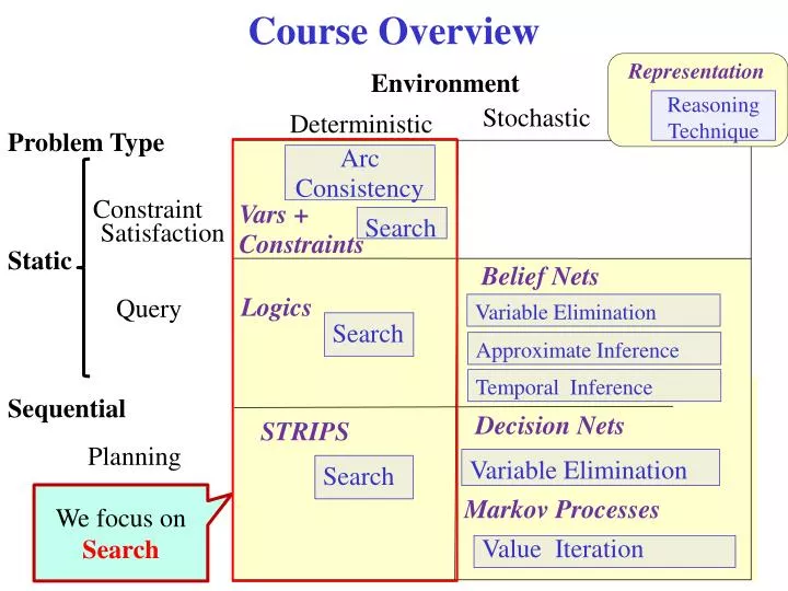
1. Course Overview Representation Reasoning Technique Stochastic Deterministic • Environment Problem Type Arc Consistency Constraint Satisfaction Vars + Constraints Search Static Belief Nets Logics Variable Elimination Query Search Approximate Inference Temporal Inference Sequential Decision Nets STRIPS Planning Variable Elimination Search We focus on Search Markov Processes Value Iteration

2. Search so far

3. A* Search • A* search takes into account both • the cost of the path to a node c(p) • the heuristic value of that path h(p). • Let f(p) = c(p) + h(p). • f(p)is an estimate of the cost of a path from the start to a goal via p. c(p) h(p) A* always chooses the path on the frontier with the lowest estimated distance from the start to a goal node constrained to go via that path. f(p)

4. Admissibility of A* • A* is complete (finds a solution, if one exists) • and optimal (finds the optimal path to a goal) if • the branching factor is finite • arc costs are > 0 • h(n) is admissible -> an underestimate of the length of the shortest path from n to a goal node. • This property of A* is called admissibility of A*

5. Why is A* admissible: complete • It finds a solution if there is one (does not get caught in cycles) • Let • fminbe the cost of the (an) optimal solution path s(unknown but finite if there exists a solution) • cmin = >0 be the minimal cost of any arc • Each sub-path p of s has f(p) ≤ fmin • Due to admissibility • A* expands path on the frontier with minimal f(n) • Always a subpath of s on the frontier • Only expands paths p with f(p) ≤ fmin • Terminates when expanding s • Because arc costs are positive, the cost of any other path p would eventually exceed fmin, at depth less no greater than (fmin / cmin ) • See how it works on the “misleading heuristic” problem in AI space:

6. Why is A* admissible: optimal • Let p*be the optimal solution path, with cost c*. • Let p’be a suboptimal solution path. That is c(p’) > c*. • We are going to show that any sub-path p’’ of p* on the frontier • will be expanded before p’ • Therefore, A* will find p* before p’ p” p’ p*

7. Analysis of A* • If fact, we can prove something even stronger about A* (when it is admissible) • A* is optimally efficient among the algorithms that • extend the search path from the initial state. • It finds the goal with the minimum # of expansions • This is because any algorithm that does not expand every node with f(n) < f* risks missing the optimal solution

8. Time Space Complexity of A* • Time complexity is O(bm) • the heuristic could be completely uninformative and the edge costs could all be the same, meaning that A* does the same thing as BFS • Space complexity is O(bm) like BFS, A* maintains a frontier which grows with the size of the tree

9. Effect of Search Heuristic • A search heuristic that is a better approximation on the actual cost reduces the number of nodes expanded by A* h2dominates h1 because h2 (n)> h1 (n) for every n Example: 8puzzle: (1) tiles can moveanywhere (h1 : number of tiles that are out of place) (2) tiles can move to any adjacent square (h2 : sum of number of squares that separate each tile from its correct position) average number of paths expanded: (d = depth of the solution) d=12 IDS = 3,644,035 paths A*(h1) = 227 paths A*(h2) = 73 paths d=24 IDS = too many paths A*(h1) = 39,135 paths A*(h2) = 1,641 paths

10. Branch-and-Bound Search • What does allow A* to do better than the other search algorithms we have seen? • What is the biggest problem with A*? • Possible Solution:

11. Branch-and-Bound Search • One way to combine DFS with heuristic guidance • Follows exactly the same search path as depth-first search • But to ensure optimality, it does not stop at the first solution found • It continues, after recording upper bound on solution cost • upper bound: UB = cost of the best solution found so far • Initialized to  or any overestimate of optimal solution cost • When a path p is selected for expansion: • Compute f(p) = cost(p) + h(p) • If f(p) UB, remove p from frontier without expanding it (pruning) • Else expand p, adding all of its neighbors to the frontier • Requires admissible h

12. Example • Arc cost = 1 • h(n) = 0 for every n • Upper Bound (UB) = ∞ Before expanding a path p, check its f value f(p): Expand only if f(p) < UB Solution! UB = ?

13. Arc cost = 1 • h(n) = 0 for every n • UB = 5 Example Cost = 5 Prune!

14. Arc cost = 1 • h(n) = 0 for every n • UB = 5 Example Solution! UB =? Cost = 5 Prune! Cost = 5 Prune!

15. Arc cost = 1 • h(n) = 0 for every n • UB = 3 Example Cost = 3 Prune! Cost = 3 Prune! Cost = 3 Prune!

16. Branch-and-Bound Analysis • Complete? • Optimal?: • Time complexity: • Space complexity:

17. Other A* Enhancements • The main problem with A* is that it uses exponential space. Branch and bound was one way around this problem, but can still get caught in infinite cycles or very long paths. • Others? • Iterative deepening A* • Memory-bounded A* • There are also ways to speed up the search via cycle checking and multiple path pruning • Study them in textbook and slides

18. Iterative Deepening A* (IDA*) • B & B can still get stuck in infinite (or extremely long) • paths • Search depth-first, but to a fixed depth, as we did for Iterative Deepening • if you don't find a solution, increase the depth tolerance and try again • depth is measured in f(n)

19. Iterative Deepening A* (IDA*) • The bound of the depth-bounded depth-first searches is in terms of f(n) • Starts at f(s): s is the start node with minimal value of h • Whenever the depth-bounded search fails unnaturally, • Start new search with bound set to the smallest f-cost of any node that exceeded the cutoff at the previous iteration • Expands same nodes as A* , but re-computes them using DFS instead of storing them

20. Analysis of Iterative Deepening A* (IDA*) • Complete and optimal? Yes, under the same conditions as A* • h is admissible • all arc costs > 0 • finite branching factor • Time complexity: O(bm) • Same argument as for Iterative Deepening DFS • Space complexity: • Same argument as for Iterative Deepening DFS • But cost of recomputing levels can be a problem in practice, if costs are real-valued. O(bm)

21. Memory-bounded A* • Iterative deepening A* and B & B use little memory • What if we have some more memory(but not enough for regular A*)? • Do A* and keep as much of the frontier in memory as possible • When running out of memory • delete worst path (highest f value) from frontier • Back the path up to a common ancestor • Subtree gets regenerated only when all other paths have been shown to be worse than the “forgotten” path

22. Memory-bounded A* • Details of the algorithm are beyond the scope of this course but • It is complete if the solution is at a depth manageable by the available memory • Optimal under the same conditions • Otherwise it returns the next best reachable solution • Often used in practice, it is considered one of the best algorithms for finding optimal solutions • It can be bogged down by having to switch back and forth among a set of candidate solution paths, of which only a few fit in memory

23. Cycle Checking and Multiple Path Pruning • Cycle checking: good when we want to avoid infinite loops, but also want to find more than one solution, if they exist • Multiple path pruning: good when we only care about finding one solution • Subsumes cycle checking

24. State space graphvs search tree k a d c b b z z k h k k c h c b a d f c b f State space graph represents the states in a given search problem, and how they are connected by the available operators Search Tree: Shows how the search space is traversed by a given search algorithm: explicitly “unfolds” the paths that are expanded. If there are cycles or multiple paths, the two look very different

25. Size of state space vs. search tree If there are cycles or multiple paths, the two look very different A A B B B C C C C C D D D • With cycles or multiple parents, the search tree can be exponential in the state space • E.g. state space with 2 actions from each state to next • With d + 1 states, search tree has depth d • 2d possible paths through the search space => exponentially larger search tree!

26. Cycle Checking • You can prune a node n that is on the path from the start node to n. • This pruning cannot remove an optimal solution => cycle check • What is the computational cost of cycle checking? • Using depth-first methods, with the graph explicitly stored, this can be done in constant time • Only one path being explored at a time • Other methods: cost is linear in path length • (check each node in the path)

27. Cycle Checking • See how DFS and BFS behave when • Search Options-> Pruning -> Loop detection • is selected • Set N1 to be a normal node so that there is only one start node. • Check, for each algorithm, what happens during the first expansion from node 3 to node 2

28. Multiple Path Pruning n • If we only want one path to the solution • Can prune path to a node n that has already been reached via a previous path • Store S := {all nodes n that have been expanded} • For newly expanded path p = (n1,…,nk,n) • Check whether n  S • Subsumes cycle check

29. Multiple Path Pruning n • See how it works by • Running BFS on the Cyclic Graph Example in CISPACE • See how it handles the multiple paths from N0 to N2 • You can erase start node N1 to simplify things

30. Multiple-Path Pruning & Optimal Solutions • Problem: what if a subsequent path to n is shorter than the first path to n, and we want an optimal solution ? • Can remove all paths from the frontier that use the longer path: these can’t be optimal. • Can change the initial segment of the paths on the frontier to use the shorter • Or… 2 2 1 1 1

31. Recap (Must Know How to Fill This ** Needs conditions

32. Algorithms Often Used in Practice ** Needs conditions

33. Search in Practice (cont’) NO Informed? Y Y Many paths to solution, no ∞ paths? NO Y Large branching factor? NO

34. Search in Practice (cont’) IDS NO B&B Informed? Y Y IDA* Many paths to solution, no ∞ paths? NO Y Large branching factor? NO MBA*

35. Sample A* applications • An Efficient A* Search Algorithm For Statistical Machine Translation. 2001 • The Generalized A* Architecture. Journal of Artificial Intelligence Research (2007) • Machine Vision … Here we consider a new compositional model for finding salient curves. • Factored A*search for models over sequences and trees International Conference on AI. 2003 • It starts saying… The primary challenge when using A* search is to find heuristic functions that simultaneously are admissible, close to actual completion costs, and efficient to calculate… • applied to NLP and BioInformatics

36. Search Summary • Search is a key computational mechanism in many AI agents • We studies the basic principles of search on the simple deterministic planning agent model • Generic search approach: • define a search space graph, • start from current state, • incrementally explore paths from current state until goal state is reached. • The way in which the frontier is expanded defines the search strategy.

37. Learning Goals for search • Identify real world examples that make use of deterministic, goal-driven search agents • Assess the size of the search space of a given search problem. • Implement the generic solution to a search problem. • Apply basic properties of search algorithms: • -completeness, optimality, time and space complexity of search algorithms. • Select the most appropriate search algorithms for specific problems. • Define/read/write/trace/debug the different search algorithms we covered • Construct heuristic functions for specific search problems • Formally prove A* optimality. • Define optimally efficient