Download
1 / 62
620 likes | 628 Views
Modeling the Power Evolution of Classical Double Radio Galaxies over Cosmological Scales. PhD Defense Talk Paramita Barai Department of Physics & Astronomy Georgia State University 11 th July, 2006. Outline. Introduction, Motivation & Methodology Models of Radio Source Evolution

E N D
Modeling the Power Evolution of Classical Double Radio Galaxies over Cosmological Scales PhD Defense Talk Paramita Barai Department of Physics & Astronomy Georgia State University 11th July, 2006
Outline • Introduction, Motivation & Methodology • Models of Radio Source Evolution • Observational Samples • Multi-dimensional Monte-Carlo Simulation • Results -- Fits to Observations -- Statistical Tests • Relevant Volume Filling Fraction • Conclusions P. Barai, GSU
Radio Galaxy (RG) Structure (Cygnus A) Chris Carilli (Perley R. A., Dreher J. W. & Cowan J. J., 1984, ApJ, 285, 35L)
Fanaroff Riley Class II RG • Separation between the points of peak intensity > (½ the total size of the source) • Bright lobes & hotspot • P178 MHz > 1025 W Hz-1 sr-1 • Synchrotron radiation e-’s in lobe magnetic field • Unification paradigm for radio loud AGN FR II’s are parent population of radio loud quasars (different viewing angles) http://www.cv.nrao.edu/~abridle/images/3c219lonopt_large.jpg
Motivation & Wider Implications • To probe the impact of RGs on the cosmological history of universe • Expanding RGs affected galaxy formation & evolution during the Quasar Era (1.5 < z < 3) • Trigger star formation Rees – 1989; De-Young – 1991, Gopal-Krishna & Wiita – 2001 • Spread metals and magnetic field into IGM • How much volume of the Relevant Universe (baryonic filaments only) do radio lobes occupy? P. Barai, GSU
Relevant Universe (WHIM) • Filaments containing baryonic material • 105 < T < 107 K • Relevant Volume as a fraction of total Volume of Universe • 0.03 @ z = 2 (Quasar era) • 0.1 @ z = 0 • Fig – Spatial distribution of warm / hot gas in the universe at present epoch -- Cen & Ostriker, 1999, ApJ, 514, 1 P. Barai, GSU
Goal / Aim • Model the individual & cosmological evolution of RGs • Estimate the Relevant Volume Fraction of the universe filled by radio lobes cumulatively over the QE P. Barai, GSU
Procedures • Semi-analytical models for RG dynamics & power evolution • Compare model predictions with observations • Extensive statistical tests quantifying the success of a model in predicting RG evolution • Choose best model, estimate physical implications Compare model predictions with observations • Virtual (pseudo) Radio Surveys -- Monte Carlo Simulations
Models • Dynamics: Kaiser & Alexander 1997, MNRAS, 286, 215 • Power: KDA: Kaiser, Dennett-Thorpe & Alexander 1997, MNRAS, 292, 723 BRW: Blundell, Rawlings & Willott 1999, AJ, 117, 677 MK: Manolakou & Kirk 2002, A&A, 391, 127 K2000: Kaiser 2000, A&A, 362, 447 BRW-modified: Vary hotspot size MK-modified: Vary hotspot size KDA-modified: Vary axial ratio P. Barai, GSU
Simplified Model of a Radio Source Kaiser C. R. & Alexander P., 1997, MNRAS, 286, 215 P. Barai, GSU
Ambient medium power-law density profile BRW & MK 0 = 1.6710–23 kg m–3 = 1.5 a0 = 10 kpc KDA 0 = 7.210–22 kg m–3 = 1.9 a0 = 2 kpc Size / Total separation between hotspots t : Age of source Q0 : Power of each jet Radio Galaxy Dynamical Evolution P. Barai, GSU
Jets move out from AGN & accelerate particles (e–' s) at termination shocks Transport of relativistic particles from head to lobe, where they emit (in radio) via synchrotron mechanism BUT key aspects of the models are different Each model ~ 10 parameters Power Losses Adiabatic loss (as source expands) Inverse Compton scattering off CMB photons Synchrotron radiation Shared Physics Adiabatic Synchrotron I.C.
Variations in the Models • Energy distribution • KDA, MK: Single power-law • BRW: break frequencies • Adiabatic loss • KDA: h.s. pressure with t • BRW: Constant h.s. size • MK: Ad. losses in head compensated (by some turbulent re-acceleration process) during transport P. Barai, GSU
Models predict the radio lobe emission Low frequency: 151 & 178 MHz Isotropic lobe emission Negligible Doppler boosting Least synchrotron / IC losses, orientation biases Redshift-complete subsamples from the flux-limited, complete radio surveys in Cambridge catalogs: 3CRR 6CE 7CRS Observables z – Redshift P151 – Specific Power at 151 MHz as in the source rest frame Dproj – Projected Linear size 151 – Spectral index at 151 MHz in the source frame [P ~ –] [z, P, D, ] Observations P. Barai, GSU
Complete Observational Samples • 3CRR – • S178 > 10.9 Jy (S151 > 12.4 Jy), 4.23 sr, 145 sources. • Declination (B1950), 10 & at 10 from galactic plane • 6CE – • 2.00 S151 3.93 Jy, 0.102 sr, 56 sources. • 08h20m30s < R.A. < 13h01m30s , +3401'00" < < +4000'00" • 7CRS – (I+II+III) • S151 > 0.5 Jy, 0.022 sr, 126 sources. • 7CI – 2h < R.A. < 2.4h , 29.5° < < 34.3° • 7CII – 8.1h < R.A. < 8.4h , 24.3° < < 29.6° • 7CIII – Within 3° radius of 18h +66° P. Barai, GSU
Radio Sky Simulation (BRW)via Multi-dimensional Monte Carlo • RG population generated from early epoch • Properties randomly drawn from distribution functions in z, jet power (Q0), age (tage) • TMaxAge = 500 Myr • Each source’s P, D evolved according to model • At tage, find what flux reaches earth now (from z) • If flux > survey limit, then RG is detected • Populations for 3C, 6C and 7C surveys from same ensemble by its size in ratio to the sky area of each survey P. Barai, GSU
Initial RG Population Generation • Jet power distribution • if, Qmin < Q0 < Qmax • Qmin = 5 1037 W • Qmax = 5 1042 W • x = 2.6 • Redshift distribution • z0 = 2.2 • z0 = 0.6 P. Barai, GSU
Radio Luminosity Function (Willott et al., 2001, MNRAS, 322, 536) • Willott et. al. FR II FR I P. Barai, GSU
Computational Work • Computationally intensive • C & IDL codes, used numerical recipes in C A single simulation • Initial ensemble size 106 – 107 50 – 200 detected in final virtual surveys • Time – several hours to days • Total no. of simulations ~ 450, by varying the parameters in search of best fit • Over 2 billion pseudo RGs were generated & evolved P. Barai, GSU
BRW-modified, MK-modified: Hot spot size grows as source ages rhs vs. L data Jeyakumar & Saikia 2000, MNRAS, 311, 397 Quadratic fit gave least reduced 2 K2000 Kaiser proposed modification to KDA: Different phead/plobe KDA-modified Increasing axial ratio Modifications to the Models P. Barai, GSU
Kolmogorov – Smirnov (K-S): Probability, (K-S) that the quantities of model and obs. are drawn from same cumulative distribution population Preliminary fig. of merit Add 1-D K-S ’s for P, D, z, for the 3 surveys in ratio of the square root of the number detected in a survey: [P, D, z, ], [P, 2D, z, ] Varied many parameters for each model to possible alternative values Statistics from several runs (with different initial random seeds) considered for each parameter variation “1-D K-S best-fit” parameters Additional Statistics 2-D K-S Test Spearman’s Partial Rank Correlation Coefficient Compare and discuss model fits Statistical Tests
“Best 1-D K-S” Results of Original Models P. Barai, GSU
“Best 1-D K-S” Results of Modified Models P. Barai, GSU
K2000 Too flat [P –D] tracks Worse statistics ([P,D,z,], [P,2D,z,]) = (1.64, 2.01) (0.241, 0.481) KDA-modified Statistics comparable to original KDA model ([P,D,z,], [P,2D,z,]) = (1.49, 2.07) (1.56, 2.10) BRW-modified Less-steep [P-D] tracks Better K-S stats after introducing growing hotspot size ([P,D,z,], [P,2D,z,] ) = (0.134, 0.142)(1.607, 1.920) MK-modified Statistics comparable to original MK model ([P,D,z,], [P,2D,z,]) = (1.95, 2.92) (1.91, 2.73) Results of Modifications P. Barai, GSU
Alternative Radio Luminosity Function • Recent RLF • Grimes, Rawlings & Willott, MNRAS, 349, 503, 2004 • z2a = 1.684 • z2b = 0.447 • KDA model (default parameters): ([P,D,z,], [P,2D,z,]) = (0.881, 0.942) (0.494, 0.690) P. Barai, GSU
Summary of Statistical Results • Models give acceptable fits for [P-D-z] distributions for Cambridge catalog subsamples • No good fit by any model or variations • K-S stat values: MK & KDA > BRW • Correlation coefficient: KDA > BRW > MK (both original & modifications) • Overall best – KDA • No single model gives excellent fit to all data simultaneously • KDA, MK, BRW-modified & MK-modified Comparable 1-D K-S statistics, better than KDA-modified & BRW • BRW-modified: Growing hotspot in BRW model Substantial improvement • KDA-modified & MK-modified comparable to / slightly better than original KDA & MK • 2-D K-S statistics Varied cases of most models can adequately fit [P-D-z] planes of surveys
Comparison of Actual & Simulated [P–D–z–] Planes(for some good cases)
Relevant Volume of the Universe • z-shell between zmin (tIN) and zmax (tOUT) • Proper volume of WHIM at zmid P. Barai, GSU