Download
1 / 29
290 likes | 301 Views
The Maturation of Nearest Neighbors Techniques. Ronald E. McRoberts Northern Research Station U.S. Forest Service St. Paul, Minnesota. Western Mensurationists Meeting 22-23 Jun 2009 Vancouver, WA. Some nearest neighbors terminology:

E N D
The Maturation of Nearest Neighbors Techniques Ronald E. McRoberts Northern Research Station U.S. Forest Service St. Paul, Minnesota Western Mensurationists Meeting 22-23 Jun 2009 Vancouver, WA
Some nearest neighbors terminology: ● Response variable: variable for which predictions are desired ● Feature space variable: ancillary variable with observation available for every population unit ● Reference set: population units with observations of both response and feature space variables ● Target set: population units for which predictions of response variables are desired
k-Nearest Neighbors {yji: j=1,…,k} is the set of k reference pixels nearest to the ith pixel in feature space with respect to a distance metric, d, Primary parameters: k, t, M
Two primary applications ● Filling holes in databases (classic imputation) - target set < reference set ● Spatial estimation - map-based inference - target set >> reference set
Issues in Nearest Neighbors prediction: ● Search for the nearest neighbors ● Search for parameter values - optimal distance metric - optimal weights {wji} - optimal k ● Inference ● Diagnostic tools
Searching for nearest neighbors k-d tree searching
Diagnostics ● Extrapolations ● Influential observations ● Preserving covariances
Diagnostic tools Ranges of feature space variables
Influential reference elements Particularly relevant when combining information from different sources; e.g., registering plot data to remotely sensed data
Diagnostic tools Preserving covariances Reference set Target set FOR VOL BA TD FOR VOL BA TD k=1 FOR 0.96 0.95 0.95 0.96 0.85 0.91 0.92 0.93 VOL 0.98 0.98 0.98 1.07 1.07 1.06 BA 0.97 0.98 1.09 1.08 TD 0.99 1.08 k=5 FOR 0.65 0.72 0.73 0.74 0.56 0.65 0.66 0.67 VOL 0.39 0.41 0.48 0.40 0.42 0.48 BA 0.43 0.48 0.44 0.49 TD 0.47 0.49
Map-based scientific inference Probability- (design-based) inference - validity based on randomization in sampling design - one and only one value for each population unit True Predicted Total C1 … Cp C1 n11 …n1p n1● … Cp np1 …npp np● Total n●1 … n●p
Inference ● Complete enumeration ● Sample-based - expression of results in probabilistic manner - typically a confidence interval - requires bias assessment - requires variance estimate
Map-based scientific inference Probability- (design-based) inference - validity based on randomization in sampling design - one and only one value for each population unit Difference estimator
Map-based scientific inference Model-based inference - validity based on model - an entire distribution of possible values for each population unit
Bias assessment ● Bootstrap ● Compare to estimates that are unbiased in expectation and asympotically unbiased
Tree density Tree count (count/ha)
Optimal distance matrix, M Find a positive, semi-definite matrix M that minimizes where nearest is defined as
Approaches: ● Canonical correlation analysis (Moeur, Stage, et al.) ● Canonical correspondence analysis (Ohmann et al.) ● Mahalanobis ● Genetic algorithm for weighted Euclidean (Tomppo et al.) ● Bayesian for full matrix (Finley et al.) ● Steepest descent (nonlinear regression) (McRoberts et al.)
Steepest descent such that m12=m21 and |M|≥0
Consequences for finding an optimal distance matrix ● surface has many local minima and maxima ● surface is very “rough” ● surface dependent on reference set ● consequences similar for any approach
Synthetic dataset: Dataset Weighted Full matrix Euclidean m22 m12=m21 m22 1 0.61 0.73 0.66 2 1.50 0.92 0.87 3 0.45 0.46 0.50 4 0.40 0.98 0.95 5 0.60 1.02 1.05
Conclusions: ● k-NN is a powerful multivariate, non-parametric technique ● efficient algorithms required for selecting parameter values ● diagnostic tools required for evaluating underlying assumptions, unbiasedness, homogeneity of variance, influential reference elements ● inferential methods required ● new thinking required for optimal distance matrix
South Savoy, Finland k Can Mah Euc Opt Cor 1 125.6 87.1 89.1 75.2 5 95.0 70.2 67.2 64.3 10 91.1 68.5 66.0 62.5 15 90.2 68.1 65.7 62.9 20 88.9 68.2 65.3 62.4 30 88.5 68.0 65.1 61.0