Download

1 / 28
280 likes | 378 Views
On Cyclic Plans for Scheduling of a Smart Card Personalisation System. Tim Nieberg Universiteit Twente, EWI/TW DWMP-Group. Overview / Objectives. Give abstract model of schedule Define (L,f)-cyclic schedule Bounds on Cycle-Time Special Schedules Tight Loading Single-Mode

E N D
On Cyclic Plans for Scheduling of a Smart Card Personalisation System Tim Nieberg Universiteit Twente, EWI/TW DWMP-Group
Overview / Objectives • Give abstract model of schedule • Define (L,f)-cyclic schedule • Bounds on Cycle-Time • Special Schedules • Tight Loading • Single-Mode • Optimal Plans for Case Study
n Smart Cards k Pers. Stations Loading/Unloading Personalisation m Graphical Machines Processing Time Conveyor Belt with n+k+2 slots underneath J1,…,Jn S1,…,Sk Pin,Pout Ppers M1,…,Mm pj pmax:= max pj Model of Personalisation System • n>1’000 • k=4,8,16,32 • ½ • 10-50 • k=5 • pPR=3 • pFO=3/2 • pL=4
Assumptions w.r.t. Case Study • For now, we assume • No time needed for placing cards onto belt • No gap b/w personalisation and graphical treatment • Flip-Over machines use single slot • Equivalent to real case • No faulty cards
(L,f)-cyclic Schedules • Definition: • A cyclic schedule that involves placing L smart cards onto the conveyor belt, and that uses f free slots, is called (L,f)-cyclic schedule. Maximizing Throughput <=> Minimizing Cycle Time
Lower Bounds on Cycle Time-> Personalisation • Consider personalisation part of system • Claim 1: • Any cyclic schedule has cycle time of at least Pin+Pout+Ppers+1. • This is the minimal time to personalise a smart card in one of the personalisation stations.
Lower Bounds on Cycle Time-> Graphical Treatment • Consider feasible, (L,f)-cyclic schedule • Belt has to advance L+f times • + Lpmax for bottleneck machine • + other f free slots under bottleneck machine • Some machine(s) have to process • maxF denotes Fth largest processing time in case that F free slots are arbitrarily presented to graphical machines M1,…,Mm • i.e.
Lower Bounds on Cycle Time-> Graphical Treatment • Claim 2: • An (L,f)-cyclic schedule has a cycle time of at least Advancement of Belt Processing Bottleneck Machine LB on Processing Non-Bottleneck
Special Schedules:Tight Loading • (k,0)-cyclic schedule • All k personalisation stations loaded and unloaded at once
Special Schedules:Tight Loading • (k,0)-cyclic schedule • All k personalisation stations loaded and unloaded at once
Special Schedules:Tight Loading • (k,0)-cyclic schedule • All k personalisation stations loaded and unloaded at once
Tight Loading: Properties • TL dominates any (L,0)-cyclic schedule • L>k: easy (split into subschedules) • L<k: yields equal or worse throughput • For the personalisation stations: • Loading is done directly after advancement of belt • Unloading occurs just before next advancement
Uniqueness of Tight Loading • Theorem 1: • Any (k,0)-cyclic schedule only loads and unloads from and to the same slot on the belt. • Idea of proof: Any other schedule results in infeasibility after insertion of at most k new cards. • Corollary: • Any other schedule uses at least one free slot per k smart cards.
(Super) Single Mode • At beginning of cycle, a free slot is inserted into system • 1.) Personalisation Station unloads if free slot is advanced underneath • 2.) Belt advances • 3.) New card is now loaded into Pers. Station • Single Mode is event-driven • Advance belt as soon as all task have been completed • Single Mode respects order of smart cards • Simple inductive arguement
(Super) Single Mode • SM defines (k,1)-cyclic schedule • When personalisation is bottleneck, i.e.Ppers+Pin+Pout > k + k pmax + max1,then SM is optimal • Pf: Claim 1 => each Pers. Station is optimally utilized.
Optimal Schedules for Case Study • Overview of bounds obtained thus far (for (k,f)-cyclic schedules): • From Claim 1:
Optimal Schedules for Case Study • Tight Loading has Cycle Time • Compare with LB
Optimal Schedules for Case Study • (k,0)-cyclic schedule does not meet bound for any Ppers > 10 in case study • By Theorem 1: • Improvement, if exist must use at least one free slot per k smart cards • => Single Mode
Optimal Plans for Case Study • Cycle Times for Single Mode
Optimal Plans for Case Study • Cycle Times for Single Mode
Optimal Plans for Case Study • Cycle Times for Single Mode
Optimal Plans for Case Study • Note that inserting even more free slots must result in plans with strictly greater cycle time
Notes on the Assumptions • Some assumptions made can be “revoked” • Loading/Unloading of conveyor belt always takes less time than bottleneck task of graphical treatment • Gap b/w Personalisation Stations and Graphical Treatment does not affect arguements presented
Conclusions • A simple characterization of cyclic schedules by the number of free slots they use has been presented • This characterization was used to show that there exists only one (k,0)-cyclic schedule (Tight Loading) • Lower bounds on the cycle time of (L,f)-cyclic schedules were given • Using destructive bounding methods, the instances of the CYBERNETIX case study were solved at optimality
Thank you for your attention… T.Nieberg@utwente.nl