Download
1 / 30
300 likes | 308 Views
All-to-All Pattern. A pattern where all (slave) processes can communicate with each other Somewhat the worst case scenario!. ITCS 4/5145 Parallel Computing, UNC-Charlotte, B. Wilkinson. slides3b.ppt Oct 14, 2014. When a pattern is repeated until some termination condition occurs.

E N D
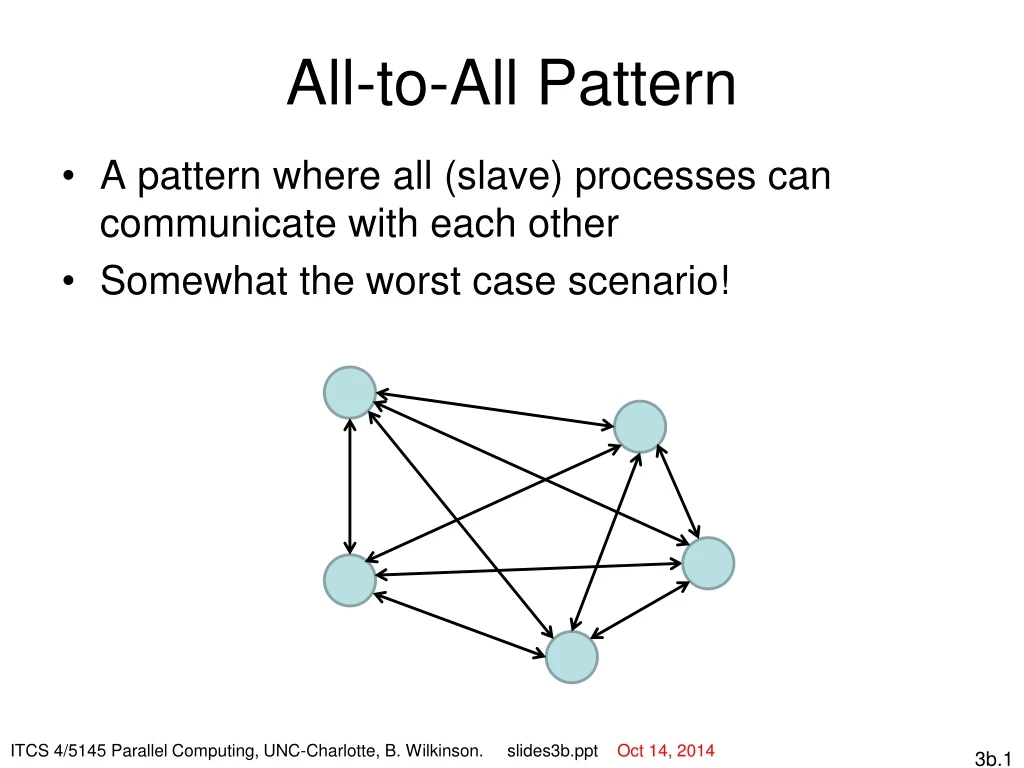
All-to-All Pattern • A pattern where all (slave) processes can communicate with each other • Somewhat the worst case scenario! ITCS 4/5145 Parallel Computing, UNC-Charlotte, B. Wilkinson. slides3b.ppt Oct 14, 2014
When a pattern is repeated until some termination condition occurs. • Synchronization at each iteration, to establish termination condition, often a global condition. • Note this is actually two patterns joined together sequentially if we call iteration a pattern. Iterative synchronous patterns Pattern Check termination condition Repeat Stop Note these pattern names are our names.
Iterative synchronous all-to-all pattern Check termination condition Repeat Stop Implemented in Seeds as the “CompleteSynchGraph” pattern. 6a.3
Application examples • N-body problem • Finding positions and movements of bodies subject to forces from other bodies. • Could be bodies such as bodies in space (gravitational N-body problem), molecular bodies fundamental particles, ... • Each iteration models one time interval. • Solving system of linear equations by iteration • Each unknown given in terms of the other unknowns • Initial guess is made for the unknowns • Iterate to converge on the solution
Gravitational N-Body Problem Finding positions and movements of bodies in space subject to gravitational forces from other bodies. Use Newtonian laws of physics: Equations: Gravitational force between two bodies of masses maand mbis: G, gravitational constant. r distance between bodies. Subject to forces, body accelerates according to Newton’s 2nd law: F = ma m is the mass of body, F force it experiences, a is the resultant acceleration.
Details Force – First compute the force: Velocity (from F=ma) Let time interval be Dt. where mass of body is m, v t+1 is velocity at time t + 1 and v tis velocity at time t. New velocity is: Position -- Over interval Dt, position changes by where xtis its position at time t. Once bodies move to new positions, forces change. Computation has to be repeated to find movement over time.
This then gives the velocity and positions in three directions.
two This then gives the velocity and positions in two directions.
Two-dimensional space -- a little easier to visualize. Movement Moves Force on body r y Another body Add the force cause by each body in x and x directions x
Code for 2-D Gravitational N-body problem Suppose a table is used to hold initial and computed data over time steps: On each iteration, position and velocities are updated. Table can be used to display movement of bodies
Sequential Code. The overall gravitational N-body computation can be described by the following steps: for (t = 0; t < tmax; t++) { //for each time period for (i = 0; i < N; i++) { //for body i, calculate force on body due to other bodies for (j = 0; j < N; j++) { if (i != j) { // for different bodies x_diff = ... ; // compute distance between body i and body j in x direction y_diff = ... ; // compute distance between body i and body j in y direction r = ... ; // compute distance r F = ... ; // compute force on bodies Fx[i] += ... ; // resolve and accumulate force in x direction Fy[i] += … ; // resolve and accumulate force in y direction } } } for (i = 0; i < N; i++) { // for each body, update positions and velocity A[i][x_velocity]= ... ; // new velocity in x direction A[i][y_velocity]= ... ; // new velocity in y direction A[i][x_position] = ... ; // new position in x direction A[i][y_position] = ... ; // new position in y direction } } // end time period
Time complexity Brute-force sequential algorithm is an O(N2) algorithm for one iteration as each of the N bodies is influenced by each of the other N - 1 bodies. For t iterations, O(N2t) Not feasible to use this direct algorithm for most interesting N-body problems where N is very large.
Reducing time complexity Time complexity can be reduced approximating a cluster of distant bodies as a single distant body with mass sited at the center of mass of the cluster:
Barnes-Hut Algorithm 3-D space: Start with whole space in which one cube contains the bodies. • First, this cube is divided into eight subcubes. • If a subcube contains no bodies, subcube deleted from further consideration. • If a subcube contains one body, subcube retained. • If a subcube contains more than one body, it is recursively divided until every subcube contains one body.
Creates an octtree - a tree with up to eight edges from each vertex (node). Leaves represent cells each containing one body. After tree constructed, total mass and center of mass of subcube stored at each vertex (node).
Force on each body obtained by traversing tree starting at root, stopping at a node when the clustering approximation can be used, e.g. when r is greater than some specified distance D. Constructing tree requires a time of O(NlogN), and so does computing all the forces, so that overall time complexity of method is O(NlogN).
Example for 2-dimensional space Construction of tree: At each vertex, store coordinates of center of mass and total mass of bodies in space below (bodies) One body
Computing force on each body -- traverse tree starting at root, stopping at a node when clustering approximation can be used, i.e. when r is greater than some set distance D. For each body Mass and coordinates of center of mass of bodies in sub space
Orthogonal Recursive Bisection An alternative way of dividing space. (For 2-dimensional area) First, a vertical line found that divides area into two areas each with equal number of bodies. For each area, a horizontal line found that divides it into two areas each with equal number of bodies. Repeated as required.
Solving General System of Linear Equations by iteration Suppose equations are of a general form with n equations and n unknowns: where the unknowns are x0, x1, x2, … xn-1 (0 <= i < n). 6a.20
By rearranging the ith equation: This equation gives xiin terms of the other unknowns. Can be used as an iteration formula for each of the unknowns to obtain better approximations. Process i computes xi 6a.21
Suppose each process computes one unknown. Pi computes xi Process Pi needs unknowns from all other processes on each iteration P0 Pn-1 (Excluding Pi) Computes: Pi Needs iterative synchronous all-to-all pattern 6a.22
Jacobi Iteration Name given to a computation that uses the previous iteration value to compute the next values. All values of x are updated together. Other (non-parallel) methods use some of the present iteration values to compute the present values, see later. 6a.23
Convergence: Can be proven that the Jacobi method will converge if diagonal values of a have an absolute value greater than sum of absolute values of other a’s on row, i.e. if This condition is a sufficient but not a necessary condition. Diagonal a’s
Termination Simple, common approach is compare values computed in one iteration to values obtained from the previous iteration. Terminate computation when all values are within given tolerance; i.e., when However, this does not guarantee the solution to that accuracy. Why? 6a.25
Convergence Rate 6a.26
Seeds “CompleteSynchGraph” Pattern All-to-all pattern that includes synchronous iteration feature to pass results of one iteration to all nodes before next iteration. Workers gets replicas of the initial data set. At each iteration, workers synchronize and update their replicas and proceed to new computations. Master node and framework will not get control of the data flow until all iterations done. More information: “Seeds Framework – The CompleteSynchGraph Template Tutorial,” Jeremy Villalobos and Yawo K. Adibolo, June 18, 2012. at http://coitweb.uncc.edu/~abw/PatternProgGroup/index.html (to be moved) Gives details with code for the Jacobi iteration method of solving system of linear equations
System of linear equations can be described in matrix-vector form: AX = B where: Possible to create an iteration formula: Xk = CXk-1 + D where Xk is solution vector at iteration k Xk-1 the solution vector at iteration k-1 C a matrix derived from input matrix A D a vector derived from input vector B. 6a.30