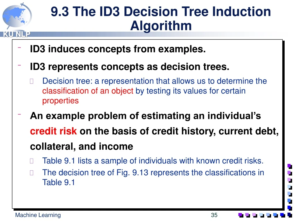
9.3 The ID3 Decision Tree Induction Algorithm

1. 9.3 The ID3 Decision Tree Induction Algorithm • ID3 induces concepts from examples. • ID3 represents concepts as decision trees. • Decision tree: a representation that allows us to determine the classification of an object by testing its values for certain properties • An example problem of estimating an individual’s credit risk on the basis of credit history, current debt, collateral, and income • Table 9.1 lists a sample of individuals with known credit risks. • The decision tree of Fig. 9.13 represents the classifications in Table 9.1 Machine Learning

2. Data from credit history of loan applications (Table 9.1) Machine Learning

3. A decision tree for credit risk assessment (Fig. 9.13) Machine Learning

4. 9.3 The ID3 Decision Tree Induction Algorithm • In a decision tree, • Each internal node represents a test on some property such as credit history or debt • Each possible value of the property corresponds to a branch of the tree such as high or low • Leaf nodes represents classifications such as low or moderate risk • An individual of unknown type may be classified by traversing the decision tree. • The size of the tree necessary to classify a given set of examples varies according to the order with which properties are tested. • Fig. 9.14 shows a tree simpler than Fig. 9.13 but the tree also classifies the examples in Table 9.1 Machine Learning

5. A simplified decision tree (Fig. 9.14) Machine Learning

6. 9.3 ID3 Decision Tree Induction Algorithm • Choice of the optimal tree • measure • the greatest likelihood of correctly classifying unseen data • assumption of ID3 algorithm • “the simplest decision tree that covers all the training examples” is the optimal tree • rationale for this assumption is time-honored heuristic of preferring simplicity & avoiding unnecessary assumptions • Occam’s Razor principle • “ It is vain to do with more what can be done with less…. Entities should not be multiplied beyond necessity ” Machine Learning

7. 9.3.1 Top-down Decision Tree Induction • ID3 algorithm • constructs decision tree in a top-down fashion • selects a property at the current node of the tree • using the property to partition the set of examples • recursively construct a subtree for each partition • Continues until all members of the partition are in the same class • Because the order of tests is critical, ID3 relies on its criteria forselecting the test • For example, ID3 constructs Fig. 9.14 from Table 9.1 • ID3 selects INCOME as the root property => Fig. 9.15 • The partition {1,4,7,11} consists entirely of high-risk and CREDIT HISTORY further devides the partition into {2,3}, {14], and {12} => Fig. 9.16 Machine Learning

8. Decision Tree Construction Algorithm Machine Learning

9. A partially constructed decision tree (Fig. 9.15) Machine Learning

10. Another partially constructed decision tree (Fig. 9.16) Machine Learning

11. 9.3.2 Information Theoretic Test Selection • Test selection method • strategy • using information theory to select the test (property) • procedure • measure the information gain • pick the property providing the greatest information gain • Information gain from property P Machine Learning

12. 9.3.2 Information Theoretic Test Selection Machine Learning

13. 9.3.2 Information Theoretic Test Selection Because INCOME provides the greatest information gain, ID3 will select it as the root. Machine Learning

14. 9.5 Knowledge and Learning • Similarity-based Learning • generalization is a function of similarities across training examples • biases are limited to syntactic constraints on the form of learned knowledge • Knowledge-based Learning • the need of prior knowledge • the most effective learning occurs when the learner already has considerable knowledge of the domain • argument for the importance of knowledge • similarity-based learning techniques rely on relatively large amount of training data. In contrast, humans can form reliable generalizations from as few as a single training instance. • any set of training examples can support an unlimited number of generalizations, most of which are irrelevant or nonsensical. Machine Learning

15. 9.5.2 Explanation-Based Learning • EBL • use an explicitly represented domain theory to construct an explanations of a training example • By generalizing from the explanation of the instance, EBL • filter noise • select relevant aspects of experience, and • organize training data into a systematic and coherent structure Machine Learning

16. 9.5.2 Explanation-Based Learning • Given • A target concept • general specification of a goal state • A training example • an instance of the target • A domain theory • a set of rules and facts that are used to explain how the training example is an instance of the goal concept • Operationality criteria • some means of describing the form that concept definitions may take • Determine • A new schema that achieves target concept in a general way Machine Learning

17. 9.5.2 Explanation-Based Learning • Example • target concept : a rule used to infer whether an object is a cup • premise(X) -> cup(X) • domain theory • liftable(X) ^ holds_liquid(X) -> cup(X) • part(Z, W) ^ concave(W) ^ points_up(W) -> holds_liquid(Z) • light(Y) ^ part(Y, handle) -> liftable(Y) • small(A) -> light(A) . made_of(A, feathers) -> light(A) • training example : an instance of the goal concept • cup(obj1) , small(obj1), part(obj1, handle), owns(bob, obj1), part(obj1, bottom), part(obj1, bowl), points_up(bowl), concave(bowl), color(obj1, red) • operationality criteria • Target concepts must be defined in terms of observable, structural properties such as part and points_up Machine Learning

18. 9.5.2 Explanation-Based Learning • Algorithm • construct an explanation of why the example is indeed an instance of the training concept (Fig. 9.17) • proof that the target concept logically follows from the example • eliminates irrelevant concepts and captures relevant concepts to the goal such as color(obj1, red) • generalize the explanation to produce a concept definition • by substituting variables for constants that are part of the training instance while retaining those constants and constraints that are part of the domain theory • EBL defines a new rule whose • conclusion is the root of the tree • premise is the conjunction of the leaves small(X) ^ part(X,handle) ^ part(X,W) ^ concave(W) ^ points_up(W) -> cup(X) Machine Learning

19. Proof that an object , X, is a cup (Fig. 9.17) Machine Learning

20. 9.5.2 Explanation-Based Learning • Benefits of EBL • select the relevant aspects of the training instance using the domain theory • form generalizations relevant to specific goals and that are guaranteed to be logically consistent with the domain theory • learning from single instance • hypothesize unstated relationships between its goals and its experience by constructing an explanation Machine Learning

21. 9.5.3 EBL and Knowledge-Level Learning • Issues in EBL • Objection • EBL cannot make the leaner do anything new • EBL only learn rules within the deductive closure of its existing theory • sole function of training instance is to focus the theorem prover on relevant aspects of the problem domain • Viewed as a form of speed up learning or knowledge base reformation • Responses to this objection • Takes information implicit in a set of rules and makes it explicit • E.g.) chess game • to focus on techniques for refining incomplete theories • development of heuristics for reasoning with imperfect theories, etc. • to focus on integrating EBL and SBL. • EBL refine training data where the theory applies • SBL further generalize the partially generalized data Machine Learning

22. 9.6 Unsupervised Learning • Supervised vs Unsupervised learning • supervised learning • the existence of a teacher, fitness function, some other external method of classifying training instances • unsupervised learning • eliminates the teacher • learner form and evaluate concepts on its own • The best example of unsupervised learning is human • Propose hypotheses to explain observations • Evaluate their hypotheses using such criteria as simplicity, generality, and elegance • Test hypotheses through experiments of their own design Machine Learning

23. 9.6.2 Conceptual Clustering • Given • a collection of unclassified objects • some means of measuring the similarity of objects • Goal • organizing the objects into a classes that meet some standard of quality, such as maximizing the similarity of objects in a class • Numeric taxonomy • The oldest approach to the clustering problem • Represent a object as a collection of features (vector of n feature values) • similarity metric : the euclidean distance between objects • Build clusters in a bottom-up fashion Machine Learning

24. 9.6.2 Conceptual Clustering • Agglomerative Clustering Algorithm • step 1 • examine all pairs of objects • select the pair with highest degree of similarity • make the pair a cluster • step 2 • define the features of the cluster as some function of the features of the component members • replace the component objects with the cluster definition • step 3 • repeat the process on the collection of objects until all objects have been reduced to a single cluster • The result of the algorithm is a binary tree whose leaf nodes are instances and whose internal nodes are clusters of increasing size Machine Learning

25. Step 0 Step 1 Step 2 Step 3 Step 4 Agglomerative (Bottom-Up) a a b b a b c d e c c d e d d e e Divisive (Top-Down) Step 3 Step 2 Step 1 Step 0 Step 4 Hierarchical Clustering • Agglomerative approachvs. Divisive approach Machine Learning

26. Agglomerative Hierarchical Clustering • 클러스터간의 유사도를 측정하는 방법 • Single-Link • 두 클러스터간의 유사도  두 클러스터에서 서로 가장 가까운 두 데이터의 유사도 • Complete-Link • 두 클러스터간의 유사도  두 클러스터에서 서로 가장 먼 두 데이터의 유사도 • Group-Averaging • Single-Link와 Complete-Link의 “Compromise” Machine Learning

27. Agglomerative Hierarchical Clustering • Single-Link : For the Good Local Coherence! Machine Learning

28. Agglomerative Hierarchical Clustering • Complete-Link: For the Good Global Cluster Quality! Machine Learning

29. Agglomerative Hierarchical Clustering • Group Averaging • Not the maximum similarity of two data from each cluster • Not the minimum similarity of two data from each cluster • Average value among all the pairs of two data from each cluster!! • Efficiency? • Single-Link Group Averaging < Complete-Link Machine Learning

30. K-means Clustering • K-means 알고리즘 Machine Learning

31. K-means Clustering • K-means 알고리즘 (cont’d) Machine Learning

32. K-means Clustering • K-means 알고리즘 • 임의로 k 개의 시작점(클러스터)을 구한다 • 각 데이터들에 대해 k개의 시작점 중 가장 가까운 점에 해당하는 클러스터로 할당한다. • 각 시작점에 할당된 데이터를 이용하여 k개의 시작점을 다시 구한다. 만일 시작점에 변화가 없으면 클러스터링을 중지한다. • 2)번을 수행한다. Machine Learning

33. K-means Clustering • K-means 알고리즘의 특징 • 빠르고 구현하기 쉽다. • k개의 점을 반드시 결정해야 한다. • “중점”을 구할 수 있는 데이터 형태에만 사용 가능하다. • 부적절한 k 값을 준다면, 엉뚱한 클러스터들이 만들어지거나 클러스터링이 완료되지 않을 수도 있다. k=4 라면? Machine Learning