Download
1 / 39
400 likes | 581 Views
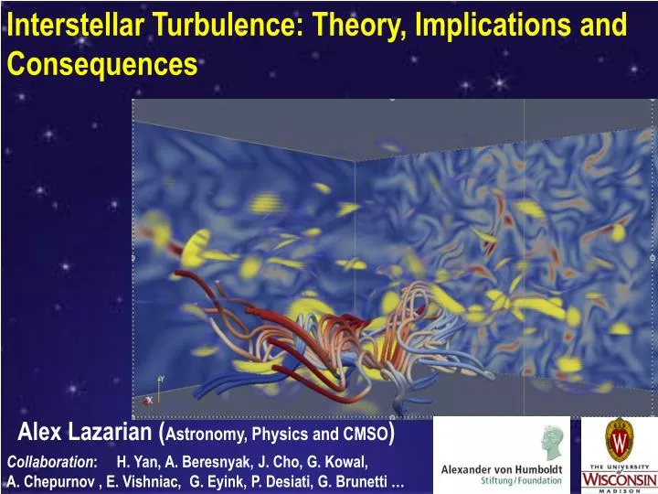
Interstellar Turbulence: Theory, Implications and Consequences. Alex Lazarian ( Astronomy, Physics and CMSO ). Collaboration : H. Yan, A. Beresnyak, J. Cho, G. Kowal, A. Chepurnov , E. Vishniac, G. Eyink, P. Desiati, G. Brunetti …. Theme 2.

E N D
Interstellar Turbulence: Theory, Implications and Consequences Alex Lazarian (Astronomy, Physics and CMSO) Collaboration: H. Yan, A. Beresnyak, J. Cho, G. Kowal, A. Chepurnov , E. Vishniac, G. Eyink, P. Desiati, G. Brunetti …
Theme 2. Propagation and Acceleration of Cosmic Rays in Turbulent Magnetic Fields
MHD turbulence theory induces changes on our understanding of CRs propagation and stochastic acceleration Highly isotropic Icecube measurement 2010 M. Duldig 2006
Points of Part 2: • Scattering and second order Fermi acceleration of cosmic rays by MHD turbulence • Perpendicular diffusion of cosmic rays • Acceleation of cosmic rays by shocks in turbulent media
Points of Part 2: • Scattering and second order Fermi acceleration of cosmic rays by MHD turbulence • Perpendicular diffusion of cosmic rays • Acceleation of cosmic rays by shocks in turbulent media
Cosmic rays interact with magnetic turbulence Cosmic Rays Magnetized medium In case of small angle scattering, Fokker-Planck equation can be used to describe the particles’ evolution: S : Sources and sinks of particles 2nd term on rhs: diffusion in phase space specified by Fokker -Planck coefficients Dxy
Correct diffusion coefficients are the key to the success of such an approach
Turbulence induces second order Fermi process Magnetic “clouds”
B rL Resonance and Transit Time Damping (TTD) are examples of 2nd order Fermi process n=1 n=0
Turbulence properties determine the diffusion and acceleration • Diffusion in the fluctuating EM fields • Collisionless Fokker-Planck equation • Boltzmann-Vlasov eq • dB, dv<<B0,V(at the scale of resonance) • Fokker-Planck coefficients: Dmm ≈ Dm2/Dt, Dpp ≈ Dp2/Dtare the • fundermental parameters we need. Those are determined by • properties of turbulence! For TTD and gyroresonance, tsc/ tac≈ Dpp / p2Dmm ≈ (VA/v)2
The diffusion coefficients define characteristics of particle propagation and acceleration ~ Propagation ~ ~ Stochastic Acceleration • The diffusion coeffecients are determined by the statistical properties of turbulence
Gyroresonance scattering depends on the properties of turbulence Gyroresonance , (n = ± 1, ± 2 …), Which states that the MHD wave frequency (Doppler shifted) is a multiple of gyrofrequency of particles (v|| is particle speed parallel to B). So, B rL
2. “steep spectrum” steeper than Kolmogorov! Less energy on resonant scale l|| l⊥ Alfenic turbulence injected at large scales is inefficient for cosmic ray scattering/acceleration 1. “random walk” 2rL B lperp<< l|| ~ rL B eddies scattering efficiency is reduced
Alfven modes (Kolmogorov) Big difference!!! Inefficiency of cosmic ray scattering by Alfvenic turbulence is obvious and contradicts to what we know about cosmic rays Scattering frequency Total path length is ~ 104 crossings at GeV from the primary to secondary ratio. (Chandran 2000) Kinetic energy Alternative solution is needed for CR scattering (Yan & Lazarian 02,04 Brunetti & Lazarian 0,).
modesmodes momodes Depends on damping Fast modes efficiently scatter cosmic rays solving problems mentioned earlier fast modes Scattering frequency plot w. linear scale Kinetic energy Fast modes are identified as the dominate source for CR scattering (Yan & Lazarian 2002, 2004).
Damping is for fast modes is usually defined for laminar fluids and is not applicable to turbulent environments Damping increases with plasma b= Pgas/Pmag and the angle q between k and B. Viscous damping (Braginskii 1965) Collisionless damping (Ginzburg 1961, Foote & Kulsrud 1979)
To calculate fast mode damping one should take into account wandering of magnetic field lines induced by Alfvenic turbulence Magnetic field wandering induced by Alfvenic turbulence was described in Lazarian & Vishniac1999 dB direction changes during cascade Field line wandering Randomization of local B: field line wandering by shearing via Alfven modes: dB/B≈ (V/L)1/2 tk1/2 Randomization of wave vector k: dk/k ≈ (kL)-1/4 V/Vph k Lazarian, Vishniac & Cho 2004 Q B Yan & Lazarian 2004
Palmer consensus from Bieber et al 1994 Modeling that accounts for damping of fast modes agrees with observations CR Transport in ISM Mean free path (pc) Text WIM halo Kinetic energy Flat dependence of mean free path can occur due to collisionless damping.
Take home message 8: • Alfvenic turbulence is inefficient for scattering if it is generated on large scales. • Fast modes dominate scattering, but damping of them is necessary to account for. • Calculation of fast mode damping requires accounting for field wandering by Alfvenic turbulence. • Scattering depends on the environment and plasma beta. • Actual turbulence and acceleration in collisionless environments may be more complex
Points of Part 2: • Scattering and second order Fermi acceleration of cosmic rays by MHD turbulence • Perpendicular diffusion of cosmic rays • Acceleation of cosmic rays by shocks in turbulent media
Perpendicular transport is due to turbulent B field • Dominated by field line wandering. B0 Intensive studies: e.g., Jokipii & Parker 1969, Forman 74, Urch 77, Bieber & Matthaeus 97, Giacolone & Jokipii 99, Matthaeus et al 03, Shalchi et al. 04 – Particle trajectory — Magnetic field What if we use the tested model of turbulence?
Perpendicular transport MA< 1, CRs free stream over distance L, thus D⊥ =R2 /∆t= Lv|| MA4 Whether and to what degree CRs diffusion is suppressed depends on Alfven Mach number, i.e MA= Vinj/VA. Lazarian & Vishniac 1999, Lazarian 2006, Yan & Lazarian 2008 Earlier works suggested MA2 dependence
Predicted MA4 suppression is observed in simulations! Xu & Yan 2013 Differs from M2 dependence in classical works, e.g. in Jokipii & Parker 69, Matthaeus et al 03.
Is Subdiffusion (∆x ~ ∝ta, a<1) typical? Subdiffusion (or compound diffusion, Getmantsev 62, Lingenfelter et al 71, Fisk et al. 73, Webb et al 06) was observed in near-slab turbulence, which can occur on small scales due to instability. What about large scale turbulence? Example: diffusion of a dye on a rope a) A rope allowing retracing, ∆t =lrope2 /D b) A rope limiting retracing within pieces lrope /n, ∆t =lrope2 /nD Diffusion is slow if particles retrace their trajectories.
Is there subdiffusion (∆x2∝∆ta, a<1) ? • Subdiffusion (or compound diffusion, Getmantsev 62, Lingenfelter et al 71, Fisk et al. 73, Webb et al 06) was observed in near-slab turbulence, which can occur on small scales due to instability. Diffusion is slow only if particles retrace their trajectories.
In turbulence, CRs’ trajactory become independent when field lines are seperated by the smallest eddy size , l⊥,min. The separation between field lines grows exponentially, provides LRR =|||,min log(l⊥,min /rL) Subdiffusion only occurs below LRR. Beyond LRR, normal diffusion applies. Subdiffusion does not happen in realistic astrophysical turbulence l||,min –Particle trajectory —Magnetic field Lazarian 06, Yan & Lazarian 08
0.01 0.01 compressible turbulence (Xu & Yan 2013 ) rL /L rL /L ∝ t ∝ t 0.001 0.001 General Normal Diffusion is observed in simulations! incompressible turbulence Beresnyak et al. (2011) Cross field transport in 3D turbulence is in general a normal diffusion!
x Xu & Yan 2013 Perpendicular propagation is superdiffusive on scales less than the injection scale Lazarian, Vishniac & Cho 2004 Magnetic field separation follows the law y2_x3 (Richarson law), x<Linj
Take home message 9: • Alfvenic Perpendicular diffusion scales as MA4, not MA2 • Subdiffusion does not happen • Superdiffusion takes place on scales smaller than the injection scale
Points of Part 2: • Scattering and second order Fermi acceleration of cosmic rays by MHD turbulence • Perpendicular diffusion of cosmic rays • Acceleation of cosmic rays by shocks in turbulent media
Point 5. Turbulence alters processes of Cosmic Ray acceleration in shocks Acceleration in shocks requires scattering of particles back from the upstream region. DownstreamUpstream Magnetic turbulence generated by shock Magnetic fluctuations generated by streaming
In postshock region damping of magnetic turbulence explains X-ray observations of young SNRs Chandra Alfvenic turbulence decays in one eddy turnover time (Cho & Lazarian 02), which results in magnetic structures behind the shock being transient andgenerating filaments of a thickness of 1016-1017cm (Pohl, Yan & Lazarian 05).
Streaming instability in the preshock region is a textbook solution for returning the particles to shock region vA B shock
B Beresnyak & Lazarian 08 Streaming instability is inefficient for producing large field in the preshock region shock Streaming instability is suppressed in the presence of external turbulence (Yan & Lazarian 02, Farmer & Goldreich 04, Beresnyak & Lazarian 08). Non-linear stage of streaming instability is inefficient (Diamond & Malkov 07).
Bell (2004) proposed a solution based on the current instability jCR B shock
Precursor forms in front of the shock and it gets turbulent as precursor interacts with gas density fluctuation
Turbulence efficiently generates magnetic fields as shown by Cho et al. 2010 hydrodynamic cascade MHD scale
The model allows to calculate the parameters of magnetic field Beresnyak, Jones & Lazarian 2010
Take home message 9: Magnetic field generated by precursor -- density fluctuations interaction might be larger than the arising from Bell’s instability current instability jCR B