Numerical Integration ( Contd )

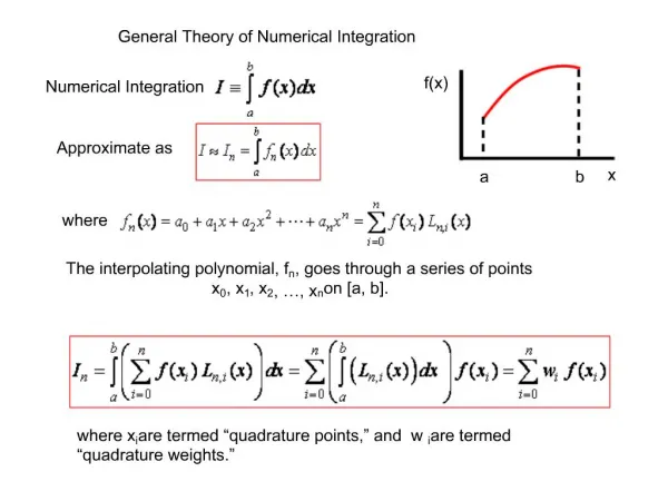
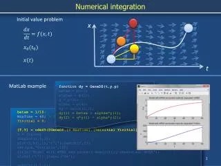
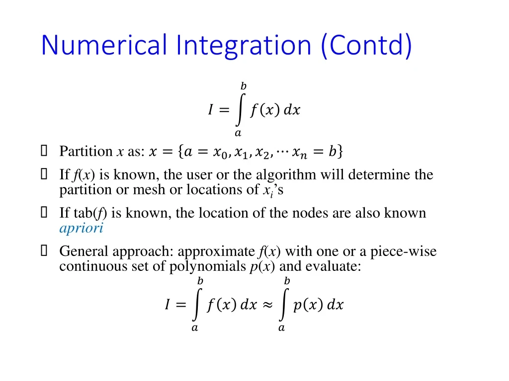
1. Numerical Integration (Contd) • Partition x as: • If f(x) is known, the user or the algorithm will determine the partition or mesh or locations of xi’s • If tab(f) is known, the location of the nodes are also known apriori • General approach: approximate f(x) with one or a piece-wise continuous set of polynomials p(x) and evaluate:

2. Numerical Integration: Rectangular Rule fi+1/2 fi+2 fn fi Polynomial p(x) is piecewise constant function: pi(x) = fi+1/2 fi+1 f1 fi-1 f0 xi+1/2 b = xn x1 a = x0 xi-1 xi+1 xi+2 xi

3. Numerical Integration: Rectangular Rule fi+1/2 fi+2 fn fi fi+1 f1 fi-1 f0 xi+1/2 b = xn x1 a = x0 xi-1 xi+1 xi+2 xi

4. Numerical Integration: Trapezoidal Rule fi+2 fn fi Polynomial p(x) is piecewise linear function: fi+1 f1 fi-1 f0 b = xn x1 a = x0 xi-1 xi+1 xi+2 xi

5. Numerical Integration: Trapezoidal Rule If the mesh is uniform, = h for all i:

6. Numerical Integration: Simpson’s Rules fi+2 fn fi Polynomial p(x) is piecewise quadratic function: fi+1 f1 fi-1 f0 b = xn x1 a = x0 xi-1 xi+1 xi+2 xi

7. Numerical Integration: Simpson’s Rules Polynomial p(x) is piecewise quadratic function: Assume, = = h and substitute z = (x – xi)

8. Numerical Integration: Simpson’s Rules Assume, = = h and substitute z = (x – xi)

9. Numerical Integration: Simpson’s Rules This is known as Simpson’s 1/3rd Rule

10. Numerical Integration: Simpson’s Rules fi+2 fn fi If the mesh is uniform, = h for all i: n = 2m, m integer fi+1 f1 fi-1 f0 b = xn x1 a = x0 xi-1 xi+1 xi+2 xi

11. Numerical Integration: Simpson’s Rules Polynomial p(x) is piecewise cubic function: Assume, = = = h and substitute z = (x – xi)

12. Numerical Integration: Simpson’s Rules This is known as Simpson’s 3/8th Rule

13. Numerical Integration: Simpson’s Rules fi+2 fn fi If the mesh is uniform, = h for all i: n = 3m, m integer fi+1 f1 fi-1 f0 b = xn x1 a = x0 xi-1 xi+1 xi+2 xi

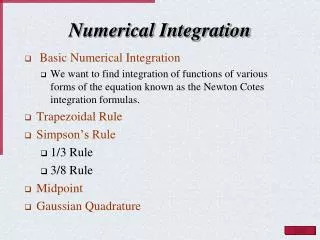
14. Numerical Integration • Accuracy: How accurate are the numerical integration schemes with respect to the TRUE integral? • Truncation Error analysis: local and global • Recall: True Value (a) = Approximate Value + Error (ε) • Is it possible to improve the accuracy? • Romberg Integration • Quadrature Methods

15. Romberg Integration

16. Gauss Quadrature All integration methods derived so far: • The weights ωi are fixed based on the method chosen! • Ability to integrate a function exactly does not depend on the number of nodes (n + 1): • Trapezoidal and Rectangular methods integrate a first order (or straight line) polynomial exactly. • Simpson’s 1/3rd rule integrates a quadratic or 2nd order polynomial exactly. • Simpson’s 3/8th rule integrates a 3rd order polynomial exactly. • For all higher order functions, there will be some error and the error is inversely proportional to n. • Goal is to design methods that can integrate a polynomial of order (2n + 1) exactly with (n + 1) nodes!

17. (a) Graphical depiction of Trapezoidal Rule (b) Improved integral estimate by taking the area under the straight line passing through two intermediate points. By positioning these points wisely, the positive and negative errors are balanced, and an improved integral estimate results Source: Chapra and Canale, pg 641 (2012)

18. Gauss Quadrature Problem: Consider the integral For a given function f(x), choose (n + 1) - xi and ωi such that the above integral is exact for a polynomial of order (2n + 1) Let f(x) be a polynomial of order (2n + 1) Let us approximate p(x) by an nth order Lagrange polynomial: Note: • the polynomial matches the function f(x) exactly at the grid points • the residual polynomial f(x) – p(x) is a polynomial of order (2n + 1) that has zeroes at the grid points.

19. Gauss Quadrature • Let g(x) be a polynomial of order (n + 1) that has zeroes at the grid points • Choose a set of linearly independent basis functionse.g., We may write:

20. Gauss Quadrature If we can choose g(x) such that, Then, and the nodes or grid points are located at the zeroes of g(x)

21. Gauss Quadrature Then, We return to choose the polynomial g(x) of order (n + 1) such that, Therefore, g(x) is a polynomial of order (n + 1) which is orthogonal to all polynomials up to order n. Two such polynomials are well-known: Legendre and Hermite

22. Gauss-Legendre Quadrature • We already know the Legendre polynomials, let’s use it! • We choose the Legendre polynomial of order (n + 1) and the zeroes of this polynomial are the nodes or grid points . Recall: • Since Legendre polynomials are defined in [-1, 1], that are also the limits of x for integrals. For arbitrary limit , use

24. Gauss-Legendre Quadrature: Example • One-point integration: • Two-points integration:

26. Gauss-Legendre Quadrature: Example • Three-points integration:

27. Numerical Integration: Example Evaluate using 3 points with Trapezoidal, Simpson’s 1/3rd and Gauss-Legendre Quadrature. Compare TRUE errors. • True integral = 26/6 = 10.6667 • Trapezoidal (T) and Simpson’s 1/3rd Rule (S): • For Gauss-Legendre Quadrature, use transformation x = (1 + z). The integral becomes:

28. Numerical Integration: Example

29. Numerical Integration: Example Consider the error function: Evaluate erf(1) using 3 points with Trapezoidal, Simpson’s 1/3rd and Gauss-Legendre Quadrature. Compare true relative errors (%) using the true erf(1) = 0.8427 • Trapezoidal (T) and Simpson’s 1/3rd Rule (S):

30. Numerical Integration: Example I