Download
1 / 52
800 likes | 1.73k Views
PART 7 Ordinary Differential Equations ODEs. Ordinary Differential Equations Part 7. Equations which are composed of an unknown function and its derivatives are called differential equations .

E N D
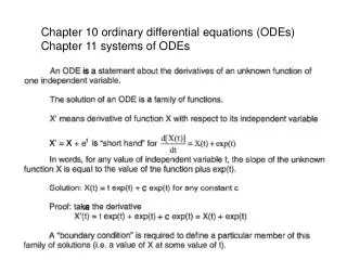
Ordinary Differential EquationsPart 7 Equations which are composed of an unknown function and its derivatives are called differential equations. Differential equations play a fundamental role in engineering because many physical phenomena are best formulated mathematically in terms of their rate of change. v - dependent variable t - independent variable
Ordinary Differential Equations • When a function involves one dependent variable, the equation is called an ordinary differential equation (ODE). • A partial differential equation(PDE)involves two or more independent variables.
Ordinary Differential Equations • Differential equations are also classified as to their order: • A first order equation includes a first derivative as its highest derivative. • - Linear 1st order ODE • - Non-Linear 1st order ODE
Ordinary Differential Equations • A second order equation includes a second derivative. • - Linear 2nd order ODE • - Non-Linear 2nd order ODE • Higher order equations can be reduced to a system of first order equations, by redefining a variable.
Runge-Kutta Methods • This chapter is devoted to solving ODE of the form: • Euler’s Method • solution
Euler’s Method: Example Obtain a solution between x = 0 to x = 4 with a step size of 0.5 for: Initial conditions are: x = 0 to y = 1 Solution:
Euler’s Method: Example • Although the computation captures the general trend solution, the error is considerable. • This error can be reduced by using a smaller step size.
System of Ordinary Differential Equations The solution is finding y1, y2,y3,…yn
Euler’s Method: Example Obtain a solution between x= 0 & 4 (step size of 0.5) Initial conditions are: x =0 ; y1= 4 & y2 = 6 Solution: X y1 y2 0 4 6 0.5 3 6.9 1 2.25 7.715 1.5 1.687 8.44525 2 1.265628 9.094087
Improvements of Euler’s method • A fundamental source of error in Euler’s method is that the derivative at the beginning of the interval is assumed to apply across the entire interval. • Simple modifications are available: • Heun’s Method • The Midpoint Method • Ralston’s Method
Runge-Kutta Methods • Runge-Kutta methods achieve the accuracy of a Taylor series approach without requiring the calculation of higher derivatives. Increment function (representative slope over the interval)
Runge-Kutta Methods • Various types of RK methods can be devised by employing different number of terms in the increment function as specified by n. • First order RK method with n=1 is Euler’s method. • Second order RK methods: • Values of a1, a2, p1, and q11 are evaluated by setting the second order equation to Taylor series expansion to the second order term.
Three equations to evaluate the four unknowns constants are derived: Runge-Kutta Methods A value is assumed for one of the unknowns to solve for the other three.
We can choose an infinite number of values for a2,there are an infinite number of second-order RK methods. Every version would yield exactly the same results if the solution to ODE were quadratic, linear, or a constant. However, they yield different results if the solution is more complicated (typically the case). Runge-Kutta Methods
Runge-Kutta Methods Three of the most commonly used methods are: • Huen Method with a Single Corrector (a2=1/2) • The Midpoint Method (a2= 1) • Raltson’s Method (a2= 2/3)
Heun’s Method: Involves the determination of two derivatives for the interval at the initial point and the end point. y f(xi+h,yi+k1h) f(xi,yi) x xi xi+h y ea Slope: 0.5(k1+k2) x xi xi+h Runge-Kutta Methods
Heun’s Method - Example Obtain a solution between x=0 & 4 (step size = 0.5) for: Initial conditions are: x = 0 to y = 1,use Heun’s method Chapter 25
y f(xi+h/2,yi+k1h/2) f(xi,yi) x xi xi+h/2 y ea Slope: k2 x xi xi+h Runge-Kutta Methods • Midpoint Method: • Uses Euler’s method t predict a value of y at the midpoint of the interval: Chapter 25
Midpoint Method (Example 25.6, P705) Obtain a solution between x=0 & 4 (step size = 0.5) for: Initial conditions are: x = 0 to y = 1,use Midpoint method Chapter 25
y f(xi,yi) xi xi+3/4h y ea Slope: (1/3k1+2/3k2) xi Runge-Kutta Methods • Ralston’s Method: f(xi+ 3/4 h, yi+3/4k1h) x xi+h x Chapter 25
Runge-Kutta Methods • Third order RK methods Chapter 25
Runge-Kutta Methods • Fourth order RK methods Chapter 25
Comparison of Runge-Kutta Methods Use first to fourth order RK methods to solve the equation from x = 0 to x = 4 Initial condition y(0) = 2, exact answer of y(4) = 75.33896 Chapter 25
y • Explicit Euler’s Method: h f(xi,yi) x y xi xi +h • Implicit Euler’s Method: f(xi+1,yi+1) f(xi,yi) h x xi xi +1 Implicit Versus Explicit Euler’s Methods Chapter 27
The Finite Difference Method • The previous central divided differences are substituted for the derivatives in the original equation. • Thus a differential equation is transformed into a set of simultaneous algebraic equations that can be solved by the methods described earlier. Chapter 27
The Central divided differences f(x) f(x) f(xi+1) f(xi-1) f(xi) f\(xi) Dx Dx x xi-1 xi xi+1 Chapter 27
The Finite Difference Method-Example Solve the following 2nd order ODE for initial conditions of T(0) = T1 and T(L)= T2 Where Ta and h/ are constants. • Solution: • Using the divided differences equations: • Substitute into the original DE for d2T/dx2: Chapter 27
The Finite Difference Method-Example • Now collecting terms gives: • The above equation is now applied at each of the interior point. • The first point and the last point are specified by the boundary conditions. • So if there is 5 points (including the first and the last point) we will have 3 equations in 3 unknowns. Chapter 27
The Finite Difference Method:Example Solve the following 2nd order ODE for initial conditions of y(0) = 5 and y(10) = -1.5, Use Dx = 2 • Using the divided differences equations: Chapter 27
The Finite Difference Method: Example • Substitute into the original DE for d2y/dx2 and dy/dx: • Now collecting terms gives and substitute for Dx =2: • The above equations will be used to find the y’s at 2, 4, 6 and 8 where y(0) = 5 and y(10) = -1.5 Chapter 27
The Finite Difference Method: Example Chapter 27
The Finite Difference Method: Example • Or in a matrix format: • Now you can use for example Gauss elimination to solve these equations. Chapter 27
PART 8Partial Differential Equations PDEs Finite Difference Method Finite Element Method Chapter 29
Partial Differential Equations Chapter 29
Partial Differential Equations • A partial differential equation(PDE)involves two or more independent variables. For example: 1. Laplace equation 2. Diffusion equation 3.Wave equation Chapter 29
Partial Differential Equations1. Finite Difference Method • Similar to the ODE, central divided differences are substituted for the partial derivatives in the original equation. • Thus a partial differential equation is transformed into a set of simultaneous algebraic equations that can be solved by the methods described earlier. Chapter 29
Partial Differential Equations y i,j+1 i,j i-1,j i+1,j i,j-1 x The Central divided differences Chapter 29
Finite Difference: Elliptic Equations • Because of its simplicity and general relevance to most areas of engineering, we will use a heated plate as an example for solving elliptic PDEs. Chapter 29
Figure 29.1 Chapter 29
Figure 29.3 Chapter 29
Laplace Equation The Laplacian Difference Equations/ O[D(x)2] O[D(y)2] Laplacian difference equation. Holds for all interior points Chapter 29
Figure 29.4 Chapter 29
In addition, boundary conditions along the edges must be specified to obtain a unique solution. • The simplest case is where the temperature at the boundary is set at a fixed value, Dirichlet boundary condition. • A balance for node (1,1) is: • Similar equations can be developed for other interior points to result a set of simultaneous equations. Chapter 29
The result is a set of nine simultaneous equations with nine unknowns: Chapter 29
Partial Differential Equations:Example 1: Laplace Equation Laplace: Substitute with the Central divided differences and assuming that Dx = Dy = h
1 -4 1 1 i,j 1 Partial Differential Equations:Example 1: Laplace Equation y Finite Difference Grid At i and j: i,j+1 i,j i-1,j i+1,j i,j-1 x