Download
1 / 57
570 likes | 714 Views
Overview of HI Astrophysics. Riccardo Giovanelli. A620 - Feb 2004. The Bohr Atom. Given a hydrogenic atom of nuclear charge Ze, if the Hamiltonian depends only on r, i.e. . The wave function is. Where the R nl (r) is an expansion in Laguerre polynomials and the spherical harmonics

E N D
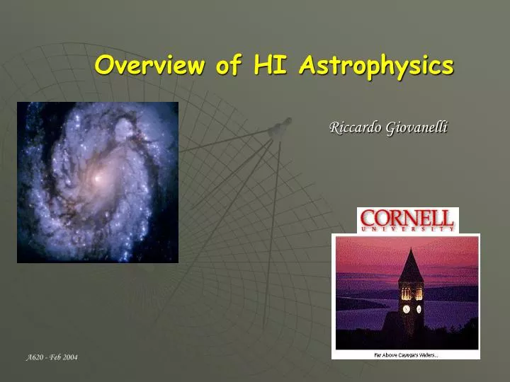
Overview of HI Astrophysics Riccardo Giovanelli A620 - Feb 2004
The Bohr Atom Given a hydrogenic atom of nuclear charge Ze, if the Hamiltonian depends only on r, i.e. The wave function is Where the Rnl(r) is an expansion in Laguerre polynomials and the spherical harmonics Ylm(q,f) are expansions of associated Legendre functions n, l and m are integer quantum numbers The bound energy levels depend only on n : Where R is Rydberg’s constant and a is the fine structure constant.
Spin-Orbit Interaction - 1 An orbiting electron is equivalent to a small current loop it produces a magnetic field of dipole moment: m =(1/c) (current in the loop) x (orbit area) = (1/c)(charge/period) x (orbit area =(1/c) (orbit area/period) x charge In an elliptical orbit, (orbit area/period) = const. = Pf/2m (Kepler’s II) so that: If we express the orbital angular momentum in units of h/2p then where is the Bohr magneton. An electron is also endowed with intrinsic SPIN, of angular momentum associated to which there is a spin magnetic moment
Spin-Orbit Interaction - 2 In the presence of a magnetic field, a dipole tends to align itself with the field. If dipole and field are misaligned, a torque is produced: In order to change the angle q, work must be done against the field: So we can ascribe a “potential energy of orientation” to a magnetic dipole in a field, i.e. different energy levels will correspond to different orientations b/w field & dipole. In a hydrogenic atom, by SPIN-ORBIT INTERACTION, we refer to that between the spin magnetic dipole of the orbiting electron and the magnetic field arising from its orbital motion. One of the consequences of the spin-orbit interaction is the Appearance of FINE STRUCTURE in the atomic energy levels.
Atomic Vector model F Total atomic angular momentum Total electronic angular momentum J Electron orbital angular momentum L I Nuclear spin angular momentum Electronic spin angular momentum S
Fine Structure The effects of relativistic corrections and the spin-orbit interaction can be treated as a perturbation term in the Hamiltonian. The resulting fine structure correction to the atomic energy levels is (Sommerfeld 1916): which for the H atom reduces to: Since i.e. considering FS a perturbation is justified
Hyperfine Structure The L-S coupling scheme leading to the fine structure correction can be applied to the interaction between the nuclear spin and the total electronic momentum. This interaction leads to the so-called “hyperfine structure” correction. As in the case of the electronic spin, the magnetic moment associated with the nuclear spin is proportional to the nuclear spin angular momentum: where the nuclear magneton is 3 orders of magnitude smaller than the Bohr magneton. While the spin-orbit (L-S) perturbation term in the Hamiltonian is The nuclear spin – electronic (I-J) perturbation term is The energy level hyperfine structure correction is (Fermi & Bethe 1933): So that:
The HI Line For the Hydrogen atom, I=1/2, so F=J+1/2 and J-1/2 For the ground state 1S1/2 (l=0, j=1/2) , the energy difference between the F=1 and f=0 energy levels is: Which corresponds to n = 1420.4058 MHz The upper level (F=1) is a triplet (2F+1=3) e and p have parallel spins The lower level (F=0) is a singlet (2F+1=1) e and p have antiparallel spins The astrophysical importance of the transition was first realized by Van de Hulst in 1944. The transition was ~ simultaneously detected in 1951 In the US, the Netehrlads and Australia (1951: Nature 168, 356).
HI Line: transition probability 1 The transition probability for spontaneous emission 1 0 is DE 0 For the 21 cm line, Hence: • The smallness of the spontaneous transition probability is due to • the fact that the transition is “forbidden” (Dl = 0) • the dependence of A10 on n3 The transition is mainly excited by other mechanisms, which make it orders of magnitude more frequent The “natural” halfwidth of the transition is 5 x 10-16 Hz
Spin Temperature If n1 and no are the population densities of atoms in levels f=1 and f=0, characterized by statistical weights g1 and go , we define Spin Temperature Ts via For the HI line, the ratio of statistical weights is 3, and hn/k=0.068 K The main excitation mechanisms for the 21 cm line are: - Collisions - Excitation by radio frequency radiation - Excitation by Lyman alpha photons Field (1958) expressed the spin temperature as a weighted average of the three: Where TR is the temperature of the radiation field at 21 cm, Tk is the kinetic temperature of the gas and TLya measures the “color” of the Ly-a radiation field
Spin Temperature- Examples • Consider a “standard” ISM cold cloud: Tk = 100K, nH = 10 cm-3 , ne = 10-3 cm-3 • where TR = TCMB = 3 K and far from HII regions: • ycoll : yLya = 350:10-5 and Ts = Tk • levels are fully regulated by collisions. • 2. Consider a warm, mainly neutral IS cloud: Tk = 5000K, nH = 0.5 cm-3, ne = 0.01 cm-3 • no nearby continuum sources, no Lyman a : • Ycoll~1.5andTs ~ 3100 K • levels still regulated by collisions but out of TE • 3. Consider the vicinity of an HII region, with high Lyman a flux: • Ts = Tk • the spin temperature is thermal, but fully regulated by the Lyman a flux.
HI Absorption coefficient Einstein Coefficients: given a two-level atom, we define three coefficients that mediate transitions between levels: - A10 probability per unit time for a spontaneous transition from 1 to 0 [s-1] - B01 multiplied by the mean intensity of the radiation field at the frequency n10 , yields the prob per u. time of absorption: 0 1 - B10 multiplied by the mean intensity of the radiation field at the frequency n10 , yields the prob per u. time of that a transition 1 0 be stimulated by an incoming photon The following relations hold: g0 B01 = g1 B10and A10 /B10 = 2hn3 /c2 Using these, it can be shown that the absorption coefficient a, defined as the fractional loss of intensity of a ray bundle travelling through unit distance within the absorbing medium, i.e. dI = - a I ds can be written as:
HI 21 cm Line transfer Consider the equation of radiative transfer: where jn is the emission coefficient and In is the specific intensity of the radiation field; by Kirchhoff’s relation: (*) Integrating (*) and introducing the optical depth t t = 0 t ‘’ I=I(0) Introducing “brightness temperature” … and if Ts is constant throughout:
HI 21 cm Line transfer-2 1. Suppose we observe a cloud of very high optical depth 2. Suppose the background radiation field is negligible ( Tb(0)~0 ) and the cloud is optically thin (t < 1). Then Recall that and to show that Then:
21cm line, optically thin case: Column density Converting frequency to velocity: where And integrating over the line profile, we obtain the cloud column density: Atoms cm-2 Where V is in km/s We assumed the background radiation to be negligible, i.e. Caveat: If Ts is comparable with TCMB, for example, then the correct expression for NH is
21cm line, optically thin case: Column density observational limits Consider a receiving system with system temperature of ~ 30 K, Integration time of 60 sec and spectral resolution of 4 km/s ~ 20 kHz; The radiometer equation yields Thus a 5-sigma detection limit will yield a minimum detectable brightness Temperature of ~ 0.14 K If we assume that the cloud “fills the beam”, and that the velocity Width of the cloud is 20 km/s, then No detections of HI in emission are known below NH~1018
21cm line, optically thin case: Column density Inverting we can write, for the optical depth at line center: Note that, for spin temperatures on order of 100K and cloud velocity widths on order of 10 km/s, for t > 1 column densities > than 1021are required Since the galactic plane is thin, face-on galaxies seldom exhibit evidence for significant optical thickness: the vast majority of the atomic gas is in optically thin clouds. As disks approach the edge-on aspect, velocity spread to a large extent prevents optical depth to increase significantly. As a result, HI masses of disk galaxies can, to first order, be inferred from The optically thin assumption.
Total HI Mass: Disk Galaxies The HI column density towards the direction (q,f) is y In c.g.s. units (freq in Hz): x If the galaxy is at distance D, then So the total nr of HI atoms in the galaxy is Where the second integral is over the solid angle subtended by the source. Converting Tb to specific intensity I, and using the definition of flux density (over)
Total HI Mass: Disk Galaxies-2 We can express: So that Converting from atomic masses to solar masses, expressing D in Mpc flux density in Jy [ 10-26 W m-2 Hz-1] and V in km/s: This is usually referred as the Flux Integral and is expressed in [ Jy km/s ] Note that this measure of HI mass will always Underestimate the true mass, since it is computed Assuming and
1940 Van de Hulst & Oort make good use of wartime 1950 1951: HI line first detected 1953: Hindman & Kerr detect HI in Magellanic Clouds Green Bank Nancay Effelsberg Parkes, J.Bank 1960 First 100 galaxies 1970 VLA and WSRT come on line Arecibo upgraded to L band; broad-band correlators, LNRs 1975: Roberts review 1977: Tully-Fisher 1980 Cluster deficiency, Synthesis maps, DLA systems, interacting systems Rotation Curves, DM, Redshift Surveys 1990 Peculiar velocity surveys, deep mapping 2000 Multifeed systems : large-scale surveys
HI Mass Function in the local Universe HI Mass Density Parkes HIPASS survey: Zwaan et al. 2003 (more from Brian on this)
Visibility of even most massive galaxies is lost at moderately low cosmic distances Low mass systems are only visible in the very local Universe. Even if abundant, we only detect a few. Parkes HIPASS Survey
Very near extragalactic space… (more later from Erik)
High Velocity Clouds ? Credit: B. Wakker
The Magellanic Stream Discovered in 1974 by Mathewson, Cleary & Murray Putman et al. 2003
ATCA map Putman et al. 1998 @ Parkes
M31 Effelsberg data Roberts, Whitehurst & Cram 1978
WSRT Map [Swaters, Sancisi & van der Hulst 1997]
A page from Dr. Bosma’s Galactic Pathology Manual [Bosma 1981]
Virgo Cluster HI Deficiency HI Disk Diameter Arecibo data [Giovanelli & Haynes 1983]
Virgo Cluster VLA data [Cayatte, van Gorkom, Balkowski & Kotanyi 1990]
VIRGO Cluster Dots: galaxies w/ measured HI Contours: HI deficiency Grey map: ROSAT 0.4-2.4 keV Solanes et al. 2002
DDO 154 Carignan & Beaulieu 1989 VLA D-array
DDO 154 Arecibo map outer extent [Hoffman et al. 1993] Extent of optical image Carignan & Beaulieu 1989 VLA D-array HI column density contours
M(total)/M(stars) M(total)/M(HI) Carignan & Beaulieu 1989
From L. van Zee’s gallery of Pathetic Galaxies (BCDs) VLA maps Van Zee & Haynes Van Zee, Skillman & Salzer Van Zee, Westphal & Haynes
NGC 3628 Leo Triplet Haynes, Giovanelli & Roberts 1979 Arecibo data NGC 3627 NGC 3623
See John Hibbard’s Gallery of Rogues at www.nrao.edu/ astrores/ HIrogues
M96 Ring Schneider et al 1989 VLA map Arecibo map Schneider, Salpeter & Terzian 19 Schneider, Helou, Salpeter & Terzian 1983
HI 1225+01 Optical galaxy Chengalur, Giovanelli & Haynes 1991 VLA data [first detected by Giovanelli, Williams & Haynes 1989 at Arecibo]
HIPASS J1712-64 7 M(HI)=1.7x10 solarm at D=3.2 Mpc V(GSR)=332 km/s …. a Magellanic ejecta HVC? Kilborn et al. 2000 Parkes discovery, ATCA map