Download

1 / 49
490 likes | 671 Views
Course Outline. Traditional Static Program Analysis Theory Compiler Optimizations; Control Flow Graphs, Data-flow Analysis Still at dataflow frameworks --- today ’ s class Examples of Analyses Class analysis Points-to analysis Applications, etc. Software Testing Dynamic Program Analysis.

E N D
Course Outline • Traditional Static Program Analysis • Theory • Compiler Optimizations; Control Flow Graphs, Data-flow Analysis • Still at dataflow frameworks --- today’s class • Examples of Analyses • Class analysis • Points-to analysis • Applications, etc. • Software Testing • Dynamic Program Analysis
Announcements • Homework 1 due Thursday • Talk at 12 to 1pm tomorrow (Tuesday) in the Biotech Auditorium • Adam Lally from IBM Watson • on Software Engineering Aspects of building the Jeopardy! system
Today • Dataflow frameworks, cont. • Monotone frameworks • The “Maximal Fixed Point” (MFP) solution • The “Meet Over all Paths” (MOP) solution • An example: What is this good for? Additional Reading: ALSU 9.3
Dataflow Lattices: Reaching Definitions U = all definitions:{(x,1),(x,4),(a,3)}The poset is 2U, ≤ is the subset relation {(x,1),(x,4),(a,3)} 1 1. x:=a*b 2. if y<=a*b {(x,1),(x,4)} {(x,4),(a,3)} {(x,1),(a,3)} 3. a:=a+1 {(x,1)} {(x,4)} {(a,3)} 4. x:=a*b 5. goto 3 0 {}
Dataflow Lattices: Available Expressions U = all expressions: {(a*b),(a+1),(y*z)}The poset is 2U, ≤ is the superset relation {} 1 1. x:=a*b 2. if y*z<=a*b {(a*b)} {(a+1)} {(y*z)} 3. a:=a+1 {(a*b),(y*z)} {(a*b),(a+1)} {(a+1),(y*z)} 4. x:=a*b 5. goto 2 0 {(a*b),(a+1),(y*z)}
Monotone Dataflow Frameworks • Framework parameters in(i)= V out(j) out(i)=Fi(in(i)) where: • in(i), out(i) are elements of a property space: • combination operator Vis U for the may problems and ∩for the must problems • set of initial values value at the nodes • Fiis the transfer function associated with node i j in pred(i)
Monotone Frameworks (cont.) • The property space must be: 1. A complete lattice (L, ≤ ) 2. L satisfies the Ascending Chain Condition (i.e., all ascending chains are finite) • The combination operator V, is the V (the join, lub) of L • The initial value at nodes is the 0 of L • Reaching Definitions: L =2U, where U is the set of all definitions in the program, and ≤ is set inclusion. • Does ACC hold for this lattice? • What is V? What is the initial value? • Available Expressions: What is (L, ≤)? Does ACC hold? What is V, initial value?
Monotone Frameworks (cont.) • The transfer functions: Fi: L L. Formally, there is space F such that • F contains all Fi, • F contains the identity function id(x) = x • F is closed under composition. 4. Each Fiis monotone.
Monotonicity • It is defined as (1) a ≤ b f(a) ≤ f(b) • An equivalent definitions is (2) f(x) V f(y) ≤ f(x V y) • Lemma: The two definitions are equivalent. First, we show that (1) implies (2). Second, we show that (2) implies (1).
Distributivity • A distributive framework: A monotone framework with distributive transfer functions: f(xV y) = f(x)Vf(y).
Framework Instances • A control flow graph CFG(N,E) • Are we propagating properties forward or backward? • A property space, what are we propagating? • A complete lattice (L,≤) • A combination operator (join, V) --- how do we merge flow? • Initial value at nodes (0 of L) --- how do we initialize nodes for fixpoint iteration • A space of monotone transfer functions F
The four classical dataflow problems Available Expressions Reaching Definitions Very Busy Expressions Live Variables LP(AExp)P(Def) P(AExp) P(Var) L,≤ is a superset is a subset is a superset is a subset L,V ∩ U ∩ U 0 AExp Ø AExp Ø ρ init(CFG) init(CFG) final(CFG) final(CFG) Initial valuesØ at ρ; 0 UNDEF; 0 Ø; 0 Ø; 0 F forward forward backward backward F {f: L L | there exist lk, lg: f(l) = (l-lk) U lg} fi fi(l) = (l - kill(i)) U gen(i)
Distributivity • Each of the four problems is an instance of a distributive framework. • First, prove monotonicity • Second, prove distributivity of the functions
Points-to Analysis: A Non-distributive Monotone Analysis • Lattice: The set of all points-to graphs Pt • ≤ is inclusion, Pt1 ≤ Pt2 if Pt1 is a subgraph of Pt2 • Transfer functions are defined on four kinds of statements: • (1) f(p=&q) is “kill” all points-to edges from p, and “generate a new points-to edge from p to q • (2) f(p=q) is “kill” all points-to edges from p, and “generate” new points-to edges from p to every x such that q points-to x • (3) f(p=*q) is “kill” all points to edges from p, and “generate” new points to edges from p to every x, such that there exists y and q points to y and y points to x • (4) f(*p=q) Do not perform kill. Can you think of a reason why? “Generate” new points-to edges from every y to every x, such that p points to y and q points to x.
A Non-distributive Monotone Example • First, we show that the framework is monotone, • I.e., for each of the four transfer functions we have to show that if Pt1 ≤ Pt2, then f(Pt1) ≤ f(Pt2) • Second, we show that the framework is not distributive • It is easy to show f(Pt1 V Pt2) ≠ f(Pt1) V f(Pt2) • Another example is constant propagation
p p q q Pt1: Pt2: x z y w p p q q f(Pt2): f(Pt1): z x w y p p q q x x y y z z w w Non-distributivity of Points-to Analysis p=&x;q=&y; p=&z;q=&w; p q Pt1 V Pt2 : x y z w What f does: Adds edges from each variable that p points to (i.e., x and z), to each variable where q points to (i.e., y and w). 4 new edges: from x to y and w, and fromz to y and w. *p=q f(Pt1) V f(Pt2) : f(Pt1 V Pt2):
Monotone Framework Instances • A control flow graph CFG(N,E) • Are we propagating properties forward or backward? • A property space, what are we propagating? • A complete lattice (L,≤) • A combination operator (join, V) --- how do we merge flow? • Initial value at nodes (0 of L) --- how do we initialize nodes for fixed point iteration • A space of monotone transfer functions F
/* Initialize to initial values */ in(1)=InitialValue; in(1) = UNDEF for m := 2 to n do in(m) := 0; in(m) := Ø W := {1,2,…,n} /* put every node on the worklist */ while W ≠ Ø do { remove i from W; out(i) = fi(in(i)); out(i) = Reach(i)∩pres(i)Ugen(i) for j in successors(i) for j in successors(i) if out(i) ≤ in(j) then { if out(i) not subset of Reach(j) in(j) = out(i) V in(j); Reach(j) = out(i) U Reach(j) if j not in W do add j to W } } The Maximal Fixed Point (MFP)1 1. The Least Fixed Point (LFP) actually…
Properties of the algorithm • Lemma1: The algorithm terminates. Sketch of the proof: We have inn(j) ≤ inn+1(j) and since L has ACC, in(j) changes at most O(h) times. Thus, each j is put on W at most O(h) times (h is the height of the lattice L). Complexity: At each iteration, the analysis examines e(j)out edges. Thus, number of basic operations is bounded by h*(e(1)out+…+e(N)out)=O(h*E). We can do better on reducible graphs.
Properties of the Algorithm • Lemma2: The algorithm computes the least solution of the dataflow equations. • For every node i MFP computes solution MFP(i) = {in(i),out(i)}, such that every other solution {in’(i),out’(i)} of the dataflow equations is “larger” than the MFP • Lemma3: The algorithm computes a correct (safe) solution.
Example Solution1 Solution2 Ø Ø inAE(1) = Ø 1. z:=x+y {(x+y)} outAE(1)= (inAE(1)-Ez) {(x+y)} {(x+y)} inAE(2) = outAE(1)Voutin(3) {(x+y)} Ø 2. if (z > 500) outAE(2)= inAE(2) {(x+y)} Ø 3. skip inAE(3) = outAE(2) outAE(3)= inAE(3) Equivalent to: inAE(2) = {(x+y)} V inAE(2) and recall that V is ∩ (i.e., set intersection). That is why we needed to initialize AEin(2) and the other initial values to the universal set of expressions (0 of the AE lattice), rather than to the more intuitive empty set.
Meet Over All Paths (MOP) Solution1 ρ n1 n2 • Desired dataflow information at n is obtained by traversing ALL PATHS from ρ to n. For every path p=(ρ, n1, n2 ..., nk) we compute fnk(…fn2(fn1(init(ρ)))) • The MOP at entry of n is Vfnk(…fn2(fn1(init(ρ)))) • The MOP is the best summary of dataflow facts possible to compute with static analysis … nk n p in paths from ρto n 1. Again, MOP is a historical name. We are taking the join…
MOP vs. MFP • For distributive functions the dataflow analysis can merge paths (p1, p2), without loss of precision! • E.g., fp1(0) need not be calculated explicitly • MFP=MOP • Due to Kam and Ullman, 1976,1977: This is not true for monotone functions. • Lemma 3: The MFP approximates the MOP for general monotone functions: MFP ≥ MOP
Function Properties • Relation of function space properties to fixed point iterative algorithms • Distributivity: • Take joins in the domain and then apply f • Apply f and then take joins in the range • The answer is the same! m1 m2 f(m1 V m2) = f(m1) V f(m2) j f(j)
Safety of Dataflow Solution • Safe (also, correct or sound) solution overestimates the best possible dataflow solution, i.e., x ≥ MOP is an approximate solution • Acceptable solution is better than what we can do with the MFP, i.e., x ≤ MFP • Between MOP and MFP are interesting solutions MFP Acceptable Safe MOP 0
Safe Solutions • In Available Expressions the 1 is the empty set, and the combination operator is set intersection. • It is safe to err by saying an expression is NOT AVAILABLE when it might be. • We compute a smaller set. Thus, under our definition of ≤, this solution is larger than the MOP. • In Reaching Definitions the 1 is the set of all (var x def) pairs. • It is safe to err by saying that a definition reaches when it DOES NOT REACH. • We compute a larger set. Thus, under our definition of ≤ (which is natural), the solution is larger than the MOP
Two Views of Reaching Definitions Defs Safe solutions are here; they are larger sets of definitions. MOP/MFP 0 element Join semi-lattice formulation. We used this formulation.
Two Views of Reaching Definitions Ø 1 element def1 … defk . . MOP/MFP Safe solutions are larger sets of definitions than MOP Defs Meet semi-lattice formulation
Kam and Ullman Results • On monotone dataflow frameworks, iterative algorithms converge to the MFP of the dataflow equations (our Lemmas 1 and 2) • MOP ≤ MFP (in our join formulation) (our Lemma 3) • One monotone framework that is not distributive is constant propagation • The MOP is undecidable for an arbitrary instance of a monotone framework.
Constant Propagation • CFG nodes are • (1) A:=B op C where A, B, C are variables and op is one of {+,-,*,/} (2) A:= integer constant • Lattice is the set of <var, ┴ / c / T> tuples (e.g, <x, ┴>, <x,5>, <y,T>. • ┴ ≤ c ≤T • ┴ means it is unknown whether a variable is a constant • c means that a variable is a constant and it is equal to c • T means that a variable is not constant • How do we define the combination operator V?
Constant Propagation • Initialization: All sets contain {<var,┴>}. At the entry point of the program we have {<var,T>}. • Transfer functions will be: fi:A:=BopC(input(i)) = output(i): • clearly, output(i) differes from input(i) only in terms of the <A,_> pair • if <B,b>,<C,c> such that b and c are constants, in input(i), then add <A,b op c> and remove any other tuples <A,_> to form output(i) • Otherwise, <A, b Vc> in output(i) fi:A:=r(input(i)) = output(i): • output(i) is formed from input(i) with <A,r> added and all previous <A,_> removed.
a:=2b:=1 a:=1b:=2 c:=a+b Constant Propagation Dataflow equations formulation (MFP): out(2) = {<a,2>,<b,1>}out(3) = {<a,1>,<b,2>}out(2) V out(3) = {<a,T>, <b,T>, <c,T>} 1 2 3 MOP formulation:f4(f2(Ø)) = f4({<a,2>,<b,1>})={<a,2>,<b,1>,<c,3>}f4(f3(Ø)) = f4({<a,1>,<b,2>})={<a,1>,<b,2>,<c,3>}f4(f2(Ø)) V f4(f3(Ø)) = {<a,T>,<b,T>,<c,3>} 4 The functions are not distributive!
a:=2b:=1 a:=1b:=2 c:=a+b Heuristic Fix • Set up dataflow equations at the exits: • out(i) =Vfj(out(j)) W = f4({<a,2>,<b,1>,<c,T>})={<a,2>,<b,1>,<c,3>} Z = f4({<a,1>,<b,2>,<c,T>})={<a,2>,<b,1>,<c,3>} Constants on exit of node 4 = W V Z={<a,T>,<b,T>,<c,3>} This only shows one can get a better approximations to the MOP, but this trick of solving on exit of nodes does not always work! 1 j in pred(i) 2 3 W Z 4
Categorizing Dataflow Problems • The four classical problems are distributive • Constant propagation is monotone, but not distributive • Points-to analysis is monotone, but not distributive
A diversion: So what is that stuff good for? • Dataflow analysis-based tools at Microsoft • The PREfix and PREfast tools • “Righting Software”, by J. Larus, T. Ball, M. Das, R. DeLine, M. Fahndrich, J. Pincus, S. Rajamani, and R. Venkatapathy in IEEE Software, 2004 • A talk by M. Beeri, Microsoft’s Haifa R&D Center, given sometimes in 2003
Static analysis tools (i.e., dataflow analysis tools) • Analyze code and detect potential defects (bugs) • Advantages: • Not limited by test cases • Identify location of bug precisely (easy to fix) • Applicable early in the development cycle • Puts responsibility on developers • Issues: • Up-front investment • Usability and noise (i.e., false warnings) • Scalability • Integration into environment
Three common questions • Do these tools (PREfix and PREfast) find important bugs? • Yes, definitely – including bugs that would cause security bulletins, blue screens, … • About 12.5% of all bugs fixed in Windows Server 2003 • Is every warning emitted by the tools useful? • No, definitely • Continued focus on “noise”, but it won’t go away • Do these tools find all the bugs? • No, no, no! • Not even all bugs of a specified kind (e.g., buffer overruns…).
PREfix • Implemented by MSR PPRC (Microsoft Research, Programmer Productivity Research Center) • C/C++ bug detection via static analysis • Powerful inter-procedural analysis • Unsound (i.e., unsafe, or ≤ MOP) • Useful in practice! • Typically run as part of a centralized build
Types of Bugs PREFix finds • Resource Leakage • Leaking Memory/Resource • Memory Management • Double free • Freeing pointer to non-allocated • memory (stack, global, etc.) • Freeing pointer in middle of memory block • Pointer Management • Dereferencing NULL pointer • Dereferencing invalid pointer • Returns pointer to local • Dereferencing or returning pointer to freed memory • Initialization • Using uninitialized memory • Freeing or dereferencing uninitialized pointer • Illegal State • Resource in illegal state • Illegal value • Divide by zero • Writing to constant string • Bounds violations • Overrun (reference beyond end) • Underflow (reference before start of buffer) • Failure to validate buffer size
PREfix Analyzer • Walks selected paths on the CFG and collects dataflow facts • Virtual machine (VIM) • Tracks the state of the dataflow facts • Finds and reports bugs based on this state • Auto Modeler (summary generator) • Generates models (i.e., summaries)of each function from collected information • E.g., function int * id(int *p) { return p; } can be modeled as follows: l = id(r); as l=r; (more on this later in class…)
PREfix example Path1: Path2: int myfunc(int j) { int k; if (j == 0) k = 1; return k; } Reserve memory Reserve memory Test: is j initialized? Evaluate j!=0 Test: is j initialized? Evaluate j==0 Def of k, k=1 Test: is k initialized? No! Report Test: is k initialized? Yes, k=1 Model (summary): Test: is actual initialized? No! Report. Test: is (actual==0)? No! Report. Note: More powerful analysis than ours. Examines (each) path, considers predicates, and does not merge flow til the end!
Analysis is unsafe! • Functions may have huge numbers of paths • PREfix only explores N paths per function • User-configurable, default is 50, usually about 100 • I.e., we give up on safety • Experiments indicate • Number of defects grows slowly with more paths: • E.g., bugs for 200 paths = 1.2 * bugs for 50 paths • E.g., bugs for 1000 paths = 1.25 * bugs for 50 paths • Analysis time grows linearly with more paths • E.g., time for 1000 paths = 20 * time for 50 paths
Analysis is imprecise (overapproximates) • Approximations for performance • E.g., loops: traverse 0 or 1 time and then approximate • E.g., recursion: explore a summary of the recursive component • Can’t always find a model for a function call • E.g., Function pointers, Virtual functions, 3rd-party party libraries • Experiments indicate relatively few spurious messages due to analysis overapproximation
Sample PREfix message void uwmsrsi4(LPCTSTR in) { TCHAR buff[100]; _tcsncpy(buff, in, sizeof(buff)); /* ... */ } TCHAR is typedef’ed as either char or wchar_t, depending on whether UNICODE is defined _tcsncpy expands to either strncpy or wcsncpy
Sample PREfix Message void uwmsrsi4(LPCTSTR in) { TCHAR buff[100]; _tcsncpy(buff, in, sizeof(buff)); /* ... */ } • uwmsrsi4.c(10) : warning 51: using number of bytes instead of number of characters for 'buff‘ used as parameter 1 (dest) of call to 'wcsncpy‘ size of 'buff' is 200 bytes reference is 399 bytes from start of buffer • uwmsrsi4.c(9) : stack variable declared hereproblem occurs when the following condition true: • uwmsrsi4.c(10) : when ‘wcslen(in) >= 200' during call to 'wcsncpy' here
Sample usage: Windows organization • PREfix: centralized runs • Bugs filed automatically • Roughly monthly from 1/2000---present (that’s at least 05) • 30M LOC – 6 days to complete a run • Some teams also run PREfix on their own • PREfast: run by individual developers/testers • Fix before check in • Or run against checked-in code in code
Summary • Detecting defects earlier in the cycle • Static analysis is becoming pervasive • PREfix, PREfast’s initial successes mean this initial successes mean this is no longer a “research” technology • Static analysis is here to stay (at least at Microsoft…) • Overcoming “noise” is vital • Technology is encouraging process change